Postprocessing

Fairlearn currently supports one postprocessing technique, ThresholdOptimizer.

Threshold optimizer

ThresholdOptimizer is based on the paper Equality of Opportunity in Supervised Learning [1]. Unlike other mitigation techniques ThresholdOptimizer is built to satisfy the specified fairness criteria exactly and with no remaining disparity. In many cases this comes at the expense of performance, for example, with significantly lower accuracy. Regardless, it provides an interesting data point for comparison with other models. Importantly, ThresholdOptimizer requires the sensitive features to be available at deployment time (i.e., for the predict method).

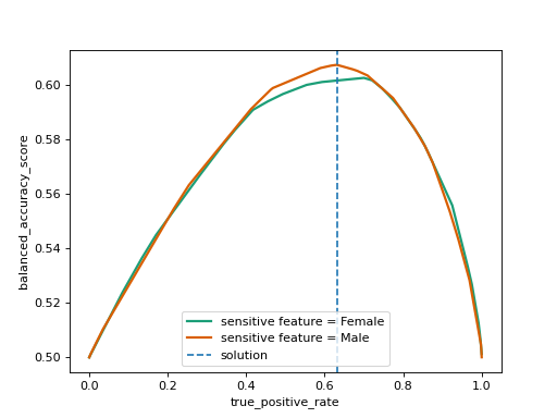
For each sensitive feature value, ThresholdOptimizer creates separate thresholds and applies them to the predictions of the user-provided estimator. To decide on the thresholds it generates all possible thresholds and selects the best combination in terms of the objective and the fairness constraints. This process is visualized below using fairlearn.postprocessing.plot_threshold_optimizer(). To ensure that the fairness constraint is upheld ThresholdOptimizer simultaneously walks along all the curves while monitoring the objective value, and picks the spot on the x-axis with the optimal objective weighed by the sizes of the groups corresponding to each sensitive feature value. The selected point is marked by the dashed blue line. The intersections with the curves are represented through interpolation of the thresholds we used to create the plot. To achieve an exact match between the sensitive feature groups in terms of the constraint, one typically needs to randomize between two thresholds.

To illustrate its behavior, let’s examine what this looks like with true positive rate parity as the fairness constraint.

>>> import json
>>> import pandas as pd
>>> from sklearn.compose import ColumnTransformer
>>> from sklearn.compose import make_column_selector as selector
>>> from sklearn.impute import SimpleImputer
>>> from sklearn.linear_model import LogisticRegression
>>> from sklearn.model_selection import train_test_split
>>> from sklearn.pipeline import Pipeline
>>> from sklearn.preprocessing import OneHotEncoder, StandardScaler
>>> from fairlearn.datasets import fetch_diabetes_hospital
>>> from fairlearn.postprocessing import ThresholdOptimizer, plot_threshold_optimizer
>>> from fairlearn.reductions import DemographicParity, ExponentiatedGradient
>>> data = fetch_diabetes_hospital(as_frame=True)
>>> # Drop 3 rows of Unknown gender since it's not representative of that group.
>>> # In a real application, this would be a red flag to investigate data collection.
>>> keep_idx = (data.data['gender'] == "Male") | (data.data['gender'] == "Female")
>>> X_raw = data.data[keep_idx]
>>> y = data.target[keep_idx]
>>> categorical_columns = [
...     'race', 'gender', 'age', 'discharge_disposition_id', 'admission_source_id',
...     'medical_specialty', 'primary_diagnosis', 'readmitted', 'max_glu_serum',
...     'A1Cresult', 'insulin', 'change', 'diabetesMed']
>>> X_raw[categorical_columns] = X_raw[categorical_columns].astype('category')
>>> # Remove readmission columns from data as they would leak the target information.
>>> X_raw.drop(columns=["readmitted", "readmit_binary"], inplace=True)
>>> A = X_raw["gender"]
>>> (X_train, X_test, y_train, y_test, A_train, A_test) = train_test_split(
...     X_raw, y, A, test_size=0.3, random_state=12345, stratify=y.astype(str) + "_" + A.astype(str))
>>> X_train = X_train.reset_index(drop=True)
>>> X_test = X_test.reset_index(drop=True)
>>> y_train = y_train.reset_index(drop=True)
>>> y_test = y_test.reset_index(drop=True)
>>> A_train = A_train.reset_index(drop=True)
>>> A_test = A_test.reset_index(drop=True)
>>> numeric_transformer = Pipeline(
...     steps=[
...         ("impute", SimpleImputer()),
...         ("scaler", StandardScaler()),
...     ]
... )
>>> categorical_transformer = Pipeline(
...     [
...         # ("impute", SimpleImputer(strategy="most_frequent")),
...         ("ohe", OneHotEncoder(handle_unknown="ignore")),
...     ]
... )
>>> preprocessor = ColumnTransformer(
...     transformers=[
...         ("num", numeric_transformer, selector(dtype_exclude="category")),
...         ("cat", categorical_transformer, selector(dtype_include="category")),
...     ]
... )
>>> pipeline = Pipeline(
...     steps=[
...         ("preprocessor", preprocessor),
...         (
...             "classifier",
...             LogisticRegression(solver="liblinear", fit_intercept=True),
...         ),
...     ]
... )
>>> threshold_optimizer = ThresholdOptimizer(
...     estimator=pipeline,
...     constraints="true_positive_rate_parity",
...     objective="balanced_accuracy_score",
...     predict_method="predict_proba",
...     prefit=False,
... )
>>> threshold_optimizer.fit(X_train, y_train, sensitive_features=A_train)
ThresholdOptimizer(constraints='true_positive_rate_parity',
                   estimator=Pipeline(steps=[('preprocessor',
                                              ColumnTransformer(transformers=[('num',
                                                                               Pipeline(steps=[('impute',
                                                                                                SimpleImputer()),
                                                                                               ('scaler',
                                                                                                StandardScaler())]),
                                                                               <sklearn.compose._column_transformer.make_column_selector object at 0x...>),
                                                                              ('cat',
                                                                               Pipeline(steps=[('ohe',
                                                                                                OneHotEncoder(handle_unknown='ignore'))]),
                                                                               <sklearn.compose._column_transformer.make_column_selector object at 0x...>)])),
                                             ('classifier',
                                              LogisticRegression(solver='liblinear'))]),
                   objective='balanced_accuracy_score',
                   predict_method='predict_proba')
>>> threshold_optimizer.predict(X_test, sensitive_features=A_test, random_state=12345)
array([0, 0, 0, ..., 0, 1, 0])
>>> threshold_rules_by_group = threshold_optimizer.interpolated_thresholder_.interpolation_dict
>>> print(json.dumps(threshold_rules_by_group, default=str, indent=4))
{
    "Female": {
        "p0": 0.628...,
        "operation0": "[>0.110...]",
        "p1": 0.371...,
        "operation1": "[>0.096...]"
    },
    "Male": {
        "p0": 0.997...,
        "operation0": "[>0.104...]",
        "p1": 0.002...,
        "operation1": "[>0.099...]"
    }
}
>>> plot_threshold_optimizer(threshold_optimizer)

When calling predict, ThresholdOptimizer uses one of the

thresholds at random based on the probabilities \(p_0\) and \(p_1\). The results can be interpreted as follows based on the following formula for the probability to predict label 1:

\[p_0 \cdot \text{operation}_0(\text{score}) + p_1 \cdot \text{operation}_1(\text{score})\]

• “Female: \(0.628 \cdot \mathbb{I}(\text{score}>0.110) + 0.371 \cdot \mathbb{I}(\text{score}>0.096)\)

  • if the score is above \(0.110\) predict 1

  • if the score is between \(0.110\) and \(0.096\) predict 1 with probability \(0.371\)

• “Male”: \(0.997 \cdot \mathbb{I}(\text{score}>0.104) + 0.002 \cdot \mathbb{I}(\text{score}>0.099)\)

  • if the score is above \(0.104\) predict 1

  • if the score is between \(0.104\) and \(0.099\) predict 1 with probability \(0.002\)

Note

The flip argument on the constructor indicates whether flipped thresholds can be used. Flipped constraints such as “<0.6” indicate that the underlying estimator’s scores do not exhibit the expected monotonicity and any such instance should be inspected.

Note

ThresholdOptimizer expects an estimator that provides it with scores. While the output of ThresholdOptimizer is binary, the input is not limited to scores derived from binary classifiers. In fact, real valued input, e.g. from a regressor, provides it with many more options to create thresholds. For \(n\) input data points with \(m \leq n\) different score values it has \(m+1\) different thresholds. At each threshold one can create one of two thresholding rules, i.e., functions that indicate which data points get label 1 based on their score.

The following combinations of fairness criteria and objectives are available:

fairness criteria	objectives
equalized_odds	accuracy_score, balanced_accuracy_score
demographic_parity, false_positive_rate_parity, false_negative_rate_parity, true_positive_rate_parity, true_negative_rate_parity	selection_rate, true_positive_rate, true_negative_rate, accuracy_score, balanced_accuracy_score

ThresholdOptimizer for equalized odds

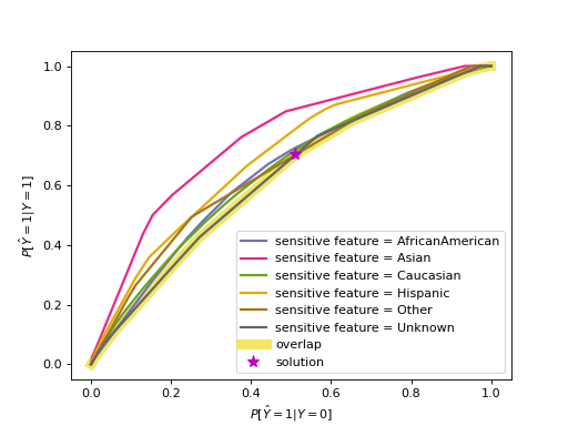
For equalized odds the behavior is somewhat different because it requires two metrics to be equal across all groups (true and false positive rate). The code below visualizes the threshold selection process with an ROC curve. The ROC curves consist of the true and false positive rates for each of the thresholding rules, with separate ones per sensitive feature value. Note that the plot omits points that are within the convex hull of points. Also note that we use race as the sensitive feature here to illustrate ROC curves that are somewhat different from each other. Using gender as we did above would result in very similar curves for the two groups.

>>> A = X_raw["race"]
>>> (X_train, X_test, y_train, y_test, A_train, A_test) = train_test_split(
...     X_raw, y, A, test_size=0.3, random_state=12345, stratify=y.astype(str) + "_" + A.astype(str))
>>> X_train = X_train.reset_index(drop=True)
>>> X_test = X_test.reset_index(drop=True)
>>> y_train = y_train.reset_index(drop=True)
>>> y_test = y_test.reset_index(drop=True)
>>> A_train = A_train.reset_index(drop=True)
>>> A_test = A_test.reset_index(drop=True)
>>> threshold_optimizer = ThresholdOptimizer(
...     estimator=pipeline,
...     constraints="equalized_odds",
...     predict_method="predict_proba",
...     objective="balanced_accuracy_score")
>>> threshold_optimizer.fit(X_train, y_train, sensitive_features=A_train)
ThresholdOptimizer(constraints='equalized_odds',
                   estimator=Pipeline(steps=[('preprocessor',
                                              ColumnTransformer(transformers=[('num',
                                                                               Pipeline(steps=[('impute',
                                                                                                SimpleImputer()),
                                                                                               ('scaler',
                                                                                                StandardScaler())]),
                                                                               <sklearn.compose._column_transformer.make_column_selector object at 0x...>),
                                                                              ('cat',
                                                                               Pipeline(steps=[('ohe',
                                                                                                OneHotEncoder(handle_unknown='ignore'))]),
                                                                               <sklearn.compose._column_transformer.make_column_selector object at 0x...>)])),
                                             ('classifier',
                                              LogisticRegression(solver='liblinear'))]),
                   objective='balanced_accuracy_score',
                   predict_method='predict_proba')
>>> threshold_rules_by_group = threshold_optimizer.interpolated_thresholder_.interpolation_dict
>>> print(json.dumps(threshold_rules_by_group, default=str, indent=4))
{
    "AfricanAmerican": {
        "p_ignore": 0.107...,
        "prediction_constant": 0.511,
        "p0": 0.987...,
        "operation0": "[>0.093...]",
        "p1": 0.012...,
        "operation1": "[>0.081...]"
    },
    "Asian": {
        "p_ignore": 0.445...,
        "prediction_constant": 0.511,
        "p0": 0.921...,
        "operation0": "[>0.084...]",
        "p1": 0.078...,
        "operation1": "[>0.066...]"
    },
    "Caucasian": {
        "p_ignore": 0.071...,
        "prediction_constant": 0.511,
        "p0": 0.708...,
        "operation0": "[>0.097...]",
        "p1": 0.291...,
        "operation1": "[>0.088...]"
    },
    "Hispanic": {
        "p_ignore": 0.311...,
        "prediction_constant": 0.511,
        "p0": 0.864...,
        "operation0": "[>0.084...]",
        "p1": 0.135...,
        "operation1": "[>0.080...]"
    },
    "Other": {
        "p_ignore": 0.0,
        "prediction_constant": 0.511,
        "p0": 0.373...,
        "operation0": "[>0.113...]",
        "p1": 0.626...,
        "operation1": "[>0.069...]"
    },
    "Unknown": {
        "p_ignore": 0.000...,
        "prediction_constant": 0.511,
        "p0": 0.183...,
        "operation0": "[>0.094...]",
        "p1": 0.816...,
        "operation1": "[>0.065...]"
    }
}
>>> plot_threshold_optimizer(threshold_optimizer)

The printed thresholding rules influence the predictions, so we need to first understand the formula that puts all the parts together. As before, to reach the optimal solution we have to interpolate between points by creating the linear combination of the two thresholds as \(p_0 \cdot \text{operation}_0(\text{score}) + p_1 \cdot \text{operation}_1(\text{score})\). The goal in this case with equalized odds is to reach equal true and false positive rates, which are conveniently plotted on the y- and x-axes, while optimizing the objective value. It follows that they’d be equal at any spot where the two curves intersect. We can relax this a little bit since in many cases one lies strictly above the other, just like in this example. Imagine the diagonal of the ROC plot from \((0,0)\) to \((1,1)\). It is usually not considered as useful since we could achieve the same result with random classifiers with probabilities to get label 1 ranging from 0 to 1. If we have one curve strictly below the other, we can still get their true and false positive rates to match by “pulling” the higher one towards the diagonal. In reality we consider the overlap, so only the points on the lower curve are available to us. From those points we choose the one with the best value in terms of the overall objective (not per group). Stepping below the Pareto curve for any sensitive feature group means introducing a probability (p_ignore) that we need to toss a biased coin whose bias is indicated by prediction_constant.

Mathematically, the following formula represents this interpretation of the chart, where \(c\) represents the prediction_constant from the printed dictionary above.

\[p_{\text{ignore}} \cdot c + (1-p_{\text{ignore}}) \cdot \left(p_0 \cdot \text{operation}_0(\text{score}) + p_1 \cdot \text{operation}_1(\text{score})\right)\]

In other words, we create a linear combination of the binary thresholding rule outputs. \(p_0\) and \(p_1\) indicate how close we are to the points representing the two thresholding rules, and \(p_0+p_1=1\). \(p_{\text{ignore}}\) is \(0\) if the curve does not need to be “pulled” towards the diagonal, i.e., when the selected solution lies on the curve itself as opposed to below. Above, the curve for “Asian” is strictly above the other curves, so \(p_{\text{ignore}}\) is highest for “Asian” and lower for other groups.

Importantly, \(p_{\text{ignore}}\) is only required for equalized odds. We want to stress on the fact that it is crucial to understand the implications of such a result. Predictions of the resulting ThresholdOptimizer model are determined randomly based on the probabilities to predict label 1 that the formula produces. Another important implication is that using randomized thresholds in this way results in what philosophers refer to as “leveling down”, i.e., decreasing performance for the better-off group without making the worse-off group any better off in absolute terms. [2] [3]

In some cases, one of the thresholds are defined to always be true or false (e.g., >-infty or <infty) resulting in base probabilities for getting a 0 or 1 regardless of the features. In our example above, this might mean that members of one group might have a base probability of being predicted to be readmitted that is higher than the base probability for members of another group. We want to emphasize that a non-zero probability to get label 1 is not acceptable in some application contexts, so it needs to be carefully evaluated whether ThresholdOptimizer should be used.

Due to the separate thresholding rules per sensitive feature value, one might argue that this constitutes disparate treatment under US anti-discrimination law or direct discrimination under EU non-discrimination law in contexts covered by these laws.

Using a pre-trained estimator

By default, ThresholdOptimizer trains the passed estimator using its fit() method. If prefit is set to True, ThresholdOptimizer does not call fit() on the estimator and assumes that it is already trained.

>>> pipeline.fit(X_train, y_train)
Pipeline(steps=[('preprocessor',
                 ColumnTransformer(transformers=[('num',
                                                  Pipeline(steps=[('impute',
                                                                   SimpleImputer()),
                                                                  ('scaler',
                                                                   StandardScaler())]),
                                                  <sklearn.compose._column_transformer.make_column_selector object at 0x...),
                                                 ('cat',
                                                  Pipeline(steps=[('ohe',
                                                                   OneHotEncoder(handle_unknown='ignore'))]),
                                                  <sklearn.compose._column_transformer.make_column_selector object at 0x...)])),
                ('classifier', LogisticRegression(solver='liblinear'))])
>>> threshold_optimizer = ThresholdOptimizer(
...     estimator=pipeline,
...     constraints="demographic_parity",
...     objective="accuracy_score",
...     prefit=True)
>>> threshold_optimizer.fit(X_train, y_train, sensitive_features=A_train)
ThresholdOptimizer(estimator=Pipeline(steps=[('preprocessor',
                                              ColumnTransformer(transformers=[('num',
                                                                               Pipeline(steps=[('impute',
                                                                                                SimpleImputer()),
                                                                                               ('scaler',
                                                                                                StandardScaler())]),
                                                                               <sklearn.compose._column_transformer.make_column_selector object at 0x...>),
                                                                              ('cat',
                                                                               Pipeline(steps=[('ohe',
                                                                                                OneHotEncoder(handle_unknown='ignore'))]),
                                                                               <sklearn.compose._column_transformer.make_column_selector object at 0x...)])),
                                             ('classifier',
                                              LogisticRegression(solver='liblinear'))]),
                   prefit=True)

If it detects that the estimator may not be fitted as defined by scikit-learn’s check it prints a warning, but still proceeds with the assumption that the user knows what they are doing. Not every machine learning package adheres to scikit-learn’s convention of setting all members with trailing underscore during fit(), so this is unfortunately an imperfect check.

References

[1]

Moritz Hardt, Eric Price, and Nati Srebro. Equality of opportunity in supervised learning. In NeurIPS, 3315–3323. 2016. URL: https://proceedings.neurips.cc/paper/2016/hash/9d2682367c3935defcb1f9e247a97c0d-Abstract.html.

[2]

Hilde Weerts, Lambèr Royakkers, and Mykola Pechenizkiy. Does the end justify the means? on the moral justification of fairness-aware machine learning. arXiv preprint arXiv:2202.08536, 2022.

[3]

Brent Mittelstadt, Sandra Wachter, and Chris Russell. The unfairness of fair machine learning: levelling down and strict egalitarianism by default. arXiv preprint arXiv:2302.02404, 2023.