Mitigation

Fairlearn contains the following algorithms for mitigating unfairness:

algorithm	description	binary classification	regression	supported fairness definitions
ExponentiatedGradient	A wrapper (reduction) approach to fair classification described in A Reductions Approach to Fair Classification 1.	✔	✔	DP, EO, TPRP, FPRP, ERP, BGL
GridSearch	A wrapper (reduction) approach described in Section 3.4 of A Reductions Approach to Fair Classification 1. For regression it acts as a grid-search variant of the algorithm described in Section 5 of Fair Regression: Quantitative Definitions and Reduction-based Algorithms 2.	✔	✔	DP, EO, TPRP, FPRP, ERP, BGL
ThresholdOptimizer	Postprocessing algorithm based on the paper Equality of Opportunity in Supervised Learning 3. This technique takes as input an existing classifier and the sensitive feature, and derives a monotone transformation of the classifier’s prediction to enforce the specified parity constraints.	✔	✘	DP, EO, TPRP, FPRP
CorrelationRemover	Preprocessing algorithm that removes correlation between sensitive features and non-sensitive features through linear transformations.	✔	✔	✘
AdversarialFairnessClassifier	An optimization algorithm based on the paper Mitigating Unwanted Biases with Adversarial Learning 4. This method trains a neural network classifier that minimizes training error while preventing an adversarial network from inferring sensitive features. The neural networks can be defined either as a PyTorch module or TensorFlow2 model.	✔	✘	DP, EO
AdversarialFairnessRegressor	The regressor variant of the above AdversarialFairnessClassifier. Useful to train a neural network with continuous valued output(s).	✘	✔	DP, EO

DP refers to demographic parity, EO to equalized odds, TPRP to true positive rate parity, FPRP to false positive rate parity, ERP to error rate parity, and BGL to bounded group loss. For more information on the definitions refer to Fairness in Machine Learning. To request additional algorithms or fairness definitions, please open a new issue on GitHub.

Note

Fairlearn mitigation algorithms largely follow the conventions of scikit-learn, meaning that they implement the fit method to train a model and the predict method to make predictions. However, in contrast with scikit-learn, Fairlearn algorithms can produce randomized predictors. Randomization of predictions is required to satisfy many definitions of fairness. Because of randomization, it is possible to get different outputs from the predictor’s predict method on identical data. For each of our algorithms, we provide explicit access to the probability distribution used for randomization.

Preprocessing

Preprocessing algorithms transform the dataset to mitigate possible unfairness present in the data. Preprocessing algorithms in Fairlearn follow the sklearn.base.TransformerMixin class, meaning that they can fit to the dataset and transform it (or fit_transform to fit and transform in one go).

Correlation Remover

Sensitive features can be correlated with non-sensitive features in the dataset. By applying the CorrelationRemover, these correlations are projected away while details from the original data are retained as much as possible (as measured by the least-squares error). The user can control the level of projection via the alpha parameter. In mathematical terms, assume we have the original dataset \(X\) which contains a set of sensitive attributes \(S\) and a set of non-sensitive attributes \(Z\). The removal of correlation is then described as:

\[\begin{split}\min _{\mathbf{z}_{1}, \ldots, \mathbf{z}_{n}} \sum_{i=1}^{n}\left\|\mathbf{z}_{i} -\mathbf{x}_{i}\right\|^{2} \\ \text{subject to} \\ \frac{1}{n} \sum_{i=1}^{n} \mathbf{z}_{i}\left(\mathbf{s}_{i}-\overline{\mathbf{s}} \right)^{T}=\mathbf{0}\end{split}\]

The solution to this problem is found by centering sensitive features, fitting a linear regression model to the non-sensitive features and reporting the residual. The columns in \(S\) will be dropped from the dataset \(X\). The amount of correlation that is removed can be controlled using the alpha parameter. This is described as follows:

\[X_{\text{tfm}} = \alpha X_{\text{filtered}} + (1-\alpha) X_{\text{orig}}\]

Note that the lack of correlation does not imply anything about statistical dependence. In particular, since correlation measures linear relationships, it might still be possible that non-linear relationships exist in the data. Therefore, we expect this to be most appropriate as a preprocessing step for (generalized) linear models.

In the example below, the Diabetes 130-Hospitals is loaded and the correlation between the African American race and the non-sensitive features is removed. This dataset contains more races, but in example we will only focus on the African American race. The CorrelationRemover will drop the sensitive features from the dataset.

>>> from fairlearn.preprocessing import CorrelationRemover
>>> import pandas as pd
>>> from sklearn.datasets import fetch_openml
>>> data = fetch_openml(data_id=43874, as_frame=True)
>>> X = data.data[["race", "time_in_hospital", "had_inpatient_days", "medicare"]]
>>> X = pd.get_dummies(X)
>>> X = X.drop(["race_Asian",
...                     "race_Caucasian",
...                     "race_Hispanic",
...                     "race_Other",
...                     "race_Unknown",
...                     "had_inpatient_days_False",
...                     "medicare_False"], axis=1)
>>> cr = CorrelationRemover(sensitive_feature_ids=['race_AfricanAmerican'])
>>> cr.fit(X)
CorrelationRemover(sensitive_feature_ids=['race_AfricanAmerican'])
>>> X_transform = cr.transform(X)

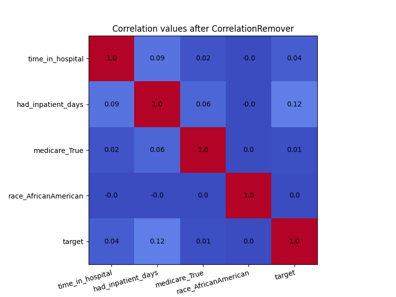
In the visualization below, we see the correlation values in the original dataset. We are particularly interested in the correlations between the ‘race_AfricanAmerican’ column and the three non-sensitive attributes ‘time_in_hospital’, ‘had_inpatient_days’ and ‘medicare_True’. The target variable is also included in these visualization for completeness, and it is defined as a binary feature which indicated whether the readmission of a patient occurred within 30 days of the release. We see that ‘race_AfricanAmerican’ is not highly correlated with the three mentioned attributes, but we want to remove these correlations nonetheless. The code for generating the correlation matrix can be found in this example notebook.

In order to see the effect of CorrelationRemover, we visualize how the correlation matrix has changed after the transformation of the dataset. Due to rounding, some of the 0.0 values appear as -0.0. Either way, the CorrelationRemover successfully removed all correlation between ‘race_AfricanAmerican’ and the other columns while retaining the correlation between the other features.

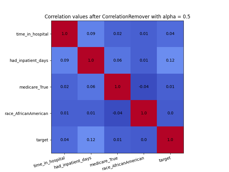
We can also use the alpha parameter with for instance \(\alpha=0.5\) to control the level of filtering between the sensitive and non-sensitive features.

>>> cr = CorrelationRemover(sensitive_feature_ids=['race_AfricanAmerican'], alpha=0.5)
>>> cr.fit(X)
CorrelationRemover(alpha=0.5, sensitive_feature_ids=['race_AfricanAmerican'])
>>> X_transform = cr.transform(X)

As we can see in the visulization below, not all correlation between ‘race_AfricanAmerican’ and the other columns was removed. This is exactly what we would expect with \(\alpha=0.5\).

Postprocessing

Reductions

On a high level, the reduction algorithms within Fairlearn enable unfairness mitigation for an arbitrary machine learning model with respect to user-provided fairness constraints. All of the constraints currently supported by reduction algorithms are group-fairness constraints. For more information on the supported fairness constraints refer to Fairness constraints for binary classification and Fairness constraints for regression.

Note

The choice of a fairness metric and fairness constraints is a crucial step in the AI development and deployment, and choosing an unsuitable constraint can lead to more harms. For a broader discussion of fairness as a sociotechnical challenge and how to view Fairlearn in this context refer to Fairness in Machine Learning.

The reductions approach for classification seeks to reduce binary classification subject to fairness constraints to a sequence of weighted classification problems (see 1), and similarly for regression (see 2). As a result, the reduction algorithms in Fairlearn only require a wrapper access to any “base” learning algorithm. By this we mean that the “base” algorithm only needs to implement fit and predict methods, as any standard scikit-learn estimator, but it does not need to have any knowledge of the desired fairness constraints or sensitive features.

From an API perspective this looks as follows in all situations

>>> reduction = Reduction(base_estimator, constraints, **kwargs)  
>>> reduction.fit(X_train, y_train, sensitive_features=sensitive_features)  
>>> reduction.predict(X_test)  

Fairlearn doesn’t impose restrictions on the referenced base_estimator other than the existence of fit and predict methods. At the moment, the base_estimator’s fit method also needs to provide a sample_weight argument which the reductions techniques use to reweight samples. In the future Fairlearn will provide functionality to handle this even without a sample_weight argument.

Before looking more into reduction algorithms, this section reviews the supported fairness constraints. All of them are expressed as objects inheriting from the base class Moment. Moment’s main purpose is to calculate the constraint violation of a current set of predictions through its gamma function as well as to provide signed_weights that are used to relabel and reweight samples.

Fairness constraints for binary classification

All supported fairness constraints for binary classification inherit from UtilityParity. They are based on some underlying metric called utility, which can be evaluated on individual data points and is averaged over various groups of data points to form the utility parity constraint of the form

\[\text{utility}_{a,e} = \text{utility}_e \quad \forall a, e\]

where \(a\) is a sensitive feature value and \(e\) is an event identifier. Each data point has only one value of a sensitive feature, and belongs to at most one event. In many examples, there is only a single event \(*\), which includes all the data points. Other examples of events include \(Y=0\) and \(Y=1\). The utility parity requires that the mean utility within each event equals the mean utility of each group whose sensitive feature is \(a\) within that event.

The class UtilityParity implements constraints that allow some amount of violation of the utility parity constraints, where the maximum allowed violation is specified either as a difference or a ratio.

The difference-based relaxation starts out by representing the utility parity constraints as pairs of inequalities

\[\begin{split}\text{utility}_{a,e} - \text{utility}_{e} \leq 0 \quad \forall a, e\\ -\text{utility}_{a,e} + \text{utility}_{e} \leq 0 \quad \forall a, e\end{split}\]

and then replaces zero on the right-hand side with a value specified as difference_bound. The resulting constraints are instantiated as

>>> UtilityParity(difference_bound=0.01)  

Note that satisfying these constraints does not mean that the difference between the groups with the highest and smallest utility in each event is bounded by difference_bound. The value of difference_bound instead bounds the difference between the utility of each group and the overall mean utility within each event. This, however, implies that the difference between groups in each event is at most twice the value of difference_bound.

The ratio-based relaxation relaxes the parity constraint as

\[r \leq \dfrac{\text{utility}_{a,e}}{\text{utility}_e} \leq \dfrac{1}{r} \quad \forall a, e\]

for some value of \(r\) in (0,1]. For example, if \(r=0.9\), this means that within each event \(0.9 \cdot \text{utility}_{a,e} \leq \text{utility}_e\), i.e., the utility for each group needs to be at least 90% of the overall utility for the event, and \(0.9 \cdot \text{utility}_e \leq \text{utility}_{a,e}\), i.e., the overall utility for the event needs to be at least 90% of each group’s utility.

The two ratio constraints can be rewritten as

\[\begin{split}- \text{utility}_{a,e} + r \cdot \text{utility}_e \leq 0 \quad \forall a, e \\ r \cdot \text{utility}_{a,e} - \text{utility}_e \leq 0 \quad \forall a, e\end{split}\]

When instantiating the ratio constraints, we use ratio_bound for \(r\), and also allow further relaxation by replacing the zeros on the right hand side by some non-negative ratio_bound_slack. The resulting instantiation looks as

>>> UtilityParity(ratio_bound=0.9, ratio_bound_slack=0.01)  

Similarly to the difference constraints, the ratio constraints do not directly bound the ratio between the pairs of groups, but such a bound is implied.

Note

It is not possible to specify both difference_bound and ratio_bound for the same constraint object.

Demographic Parity

A binary classifier \(h(X)\) satisfies demographic parity if

\[\P[h(X) = 1 \given A = a] = \P[h(X) = 1] \quad \forall a\]

In other words, the selection rate or percentage of samples with label 1 should be equal across all groups. Implicitly this means the percentage with label 0 is equal as well. In this case, the utility function is equal to \(h(X)\) and there is only a single event \(*\).

In the example below group "a" has a selection rate of 60%, "b" has a selection rate of 20%. The overall selection rate is 40%, so "a" is 0.2 above the overall selection rate, and "b" is 0.2 below. Invoking the method gamma shows the values of the left-hand sides of the constraints described in Fairness constraints for binary classification, which is independent of the provided difference_bound. Note that the left-hand sides corresponding to different values of sign are just negatives of each other. The value of y_true is in this example irrelevant to the calculations, because the underlying utility in demographic parity, selection rate, does not consider performance relative to the true labels, but rather proportions in the predicted labels.

Note

When providing DemographicParity to mitigation algorithms, only use the constructor and the mitigation algorithm itself then invokes load_data. The example below uses load_data to illustrate how DemographicParity instantiates inequalities from Fairness constraints for binary classification.

>>> from fairlearn.reductions import DemographicParity
>>> from fairlearn.metrics import MetricFrame, selection_rate
>>> import numpy as np
>>> import pandas as pd
>>> dp = DemographicParity(difference_bound=0.01)
>>> X                  = np.array([[0], [1], [2], [3], [4], [5], [6], [7], [8], [9]])
>>> y_true             = np.array([ 1 ,  1 ,  1 ,  1 ,  0,   0 ,  0 ,  0 ,  0 ,  0 ])
>>> y_pred             = np.array([ 1 ,  1 ,  1 ,  1 ,  0,   0 ,  0 ,  0 ,  0 ,  0 ])
>>> sensitive_features = np.array(["a", "b", "a", "a", "b", "a", "b", "b", "a", "b"])
>>> selection_rate_summary = MetricFrame(metrics=selection_rate,
...                                      y_true=y_true,
...                                      y_pred=y_pred,
...                                      sensitive_features=pd.Series(sensitive_features, name="SF 0"))
>>> selection_rate_summary.overall
    0.4
>>> selection_rate_summary.by_group
SF 0
a    0.6
b    0.2
Name: selection_rate, dtype: float64
>>> dp.load_data(X, y_true, sensitive_features=sensitive_features)
>>> dp.gamma(lambda X: y_pred)
sign  event  group_id
+     all    a           0.2
             b          -0.2
-     all    a          -0.2
             b           0.2
dtype: float64

The ratio constraints for the demographic parity with ratio_bound \(r\) (and ratio_bound_slack=0) take form

\[r \leq \dfrac{\P[h(X) = 1 \given A = a]}{\P[h(X) = 1]} \leq \dfrac{1}{r} \quad \forall a\]

Revisiting the same example as above we get

>>> dp = DemographicParity(ratio_bound=0.9, ratio_bound_slack=0.01)
>>> dp.load_data(X, y_pred, sensitive_features=sensitive_features)
>>> dp.gamma(lambda X: y_pred)
sign  event  group_id
+     all    a           0.14
             b          -0.22
-     all    a          -0.24
             b           0.16
dtype: float64

Following the expressions for the left-hand sides of the constraints, we obtain

\[\begin{split}r \cdot \text{utility}_{a,*} - \text{utility}_* = 0.9 \times 0.6 - 0.4 = 0.14 \\ r \cdot \text{utility}_{b,*} - \text{utility}_* = 0.9 \times 0.2 - 0.4 = -0.22 \\ - \text{utility}_{a,*} + r \cdot \text{utility}_* = - 0.6 + 0.9 \times 0.4 = -0.24 \\ - \text{utility}_{b,*} + r \cdot \text{utility}_* = - 0.2 + 0.9 \times 0.4 = 0.16 \\\end{split}\]

True Positive Rate Parity and False Positive Rate Parity

A binary classifier \(h(X)\) satisfies true positive rate parity if

\[\P[h(X) = 1 \given A = a, Y = 1] = \P[h(X) = 1 \given Y = 1] \quad \forall a\]

and false positive rate parity if

\[\P[h(X) = 1 \given A = a, Y = 0] = \P[h(X) = 1 \given Y = 0] \quad \forall a\]

In first case, we only have one event \(Y=1\) and ignore the samples with \(Y=0\), and in the second case vice versa. Refer to Equalized Odds for the fairness constraint type that simultaneously enforce both true positive rate parity and false positive rate parity by considering both events \(Y=0\) and \(Y=1\).

In practice this can be used in a difference-based relaxation as follows:

>>> from fairlearn.reductions import TruePositiveRateParity
>>> from fairlearn.metrics import true_positive_rate
>>> import numpy as np
>>> tprp = TruePositiveRateParity(difference_bound=0.01)
>>> X                  = np.array([[0], [1], [2], [3], [4], [5], [6], [7], [8], [9]])
>>> y_true             = np.array([ 1 ,  1 ,  1 ,  1 ,  1,   1 ,  1 ,  0 ,  0 ,  0 ])
>>> y_pred             = np.array([ 1 ,  1 ,  1 ,  1 ,  0,   0 ,  0 ,  1 ,  0 ,  0 ])
>>> sensitive_features = np.array(["a", "b", "a", "a", "b", "a", "b", "b", "a", "b"])
>>> tpr_summary = MetricFrame(metrics=true_positive_rate,
...                           y_true=y_true,
...                           y_pred=y_pred,
...                           sensitive_features=sensitive_features)
>>> tpr_summary.overall
0.5714285714285714
>>> tpr_summary.by_group
sensitive_feature_0
a    0.75...
b    0.33...
Name: true_positive_rate, dtype: float64
>>> tprp.load_data(X, y_true, sensitive_features=sensitive_features)
>>> tprp.gamma(lambda X: y_pred)
sign  event    group_id
+     label=1  a           0.1785...
               b          -0.2380...
-     label=1  a          -0.1785...
               b           0.2380...
dtype: float64

Note

When providing TruePositiveRateParity or FalsePositiveRateParity to mitigation algorithms, only use the constructor. The mitigation algorithm itself then invokes load_data. The example uses load_data to illustrate how TruePositiveRateParity instantiates inequalities from Fairness constraints for binary classification.

Alternatively, a ratio-based relaxation is also available:

>>> tprp = TruePositiveRateParity(ratio_bound=0.9, ratio_bound_slack=0.01)
>>> tprp.load_data(X, y_true, sensitive_features=sensitive_features)
>>> tprp.gamma(lambda X: y_pred)
sign  event    group_id
+     label=1  a           0.1035...
               b          -0.2714...
-     label=1  a          -0.2357...
               b           0.1809...
dtype: float64

Equalized Odds

A binary classifier \(h(X)\) satisfies equalized odds if it satisfies both true positive rate parity and false positive rate parity, i.e.,

\[\P[h(X) = 1 \given A = a, Y = y] = \P[h(X) = 1 \given Y = y] \quad \forall a, y\]

The constraints represent the union of constraints for true positive rate and false positive rate.

>>> from fairlearn.reductions import EqualizedOdds
>>> eo = EqualizedOdds(difference_bound=0.01)
>>> eo.load_data(X, y_true, sensitive_features=sensitive_features)
>>> eo.gamma(lambda X: y_pred)
sign  event    group_id
+     label=0  a          -0.3333...
               b           0.1666...
      label=1  a           0.1785...
               b          -0.2380...
-     label=0  a           0.3333...
               b          -0.1666...
      label=1  a          -0.1785...
               b           0.2380...
dtype: float64

Error Rate Parity

The error rate parity requires that the error rates should be the same across all groups. For a classifier \(h(X)\) this means that

\[\P[h(X) \ne Y \given A = a] = \P[h(X) \ne Y] \quad \forall a\]

In this case, the utility is equal to 1 if \(h(X)\ne Y\) and equal to 0 if \(h(X)=Y\), and so large value of utility here actually correspond to poor outcomes. The difference-based relaxation specifies that the error rate of any given group should not deviate from the overall error rate by more than the value of difference_bound.

>>> from fairlearn.reductions import ErrorRateParity
>>> from sklearn.metrics import accuracy_score
>>> accuracy_summary = MetricFrame(metrics=accuracy_score,
...                                y_true=y_true,
...                                y_pred=y_pred,
...                                sensitive_features=sensitive_features)
>>> accuracy_summary.overall
0.6
>>> accuracy_summary.by_group
sensitive_feature_0
a    0.8
b    0.4
Name: accuracy_score, dtype: float64
>>> erp = ErrorRateParity(difference_bound=0.01)
>>> erp.load_data(X, y_true, sensitive_features=sensitive_features)
>>> erp.gamma(lambda X: y_pred)
sign  event  group_id
+     all    a          -0.2
             b           0.2
-     all    a           0.2
             b          -0.2
dtype: float64

Note

When providing ErrorRateParity to mitigation algorithms, only use the constructor. The mitigation algorithm itself then invokes load_data. The example uses load_data to illustrate how ErrorRateParity instantiates inequalities from Fairness constraints for binary classification.

Alternatively, error rate parity can be relaxed via ratio constraints as

\[r \leq \dfrac{\P[h(X) \ne Y \given A = a]}{\P[h(X) \ne Y]} \leq \dfrac{1}{r} \quad \forall a\]

with a ratio_bound \(r\). The usage is identical with other constraints:

>>> from fairlearn.reductions import ErrorRateParity
>>> erp = ErrorRateParity(ratio_bound=0.9, ratio_bound_slack=0.01)
>>> erp.load_data(X, y_true, sensitive_features=sensitive_features)
>>> erp.gamma(lambda X: y_pred)
sign  event  group_id
+     all    a          -0.22
             b           0.14
-     all    a           0.16
             b          -0.24
dtype: float64

Control features

The above examples of Moment (Demographic Parity, True and False Positive Rate Parity, Equalized Odds and Error Rate Parity) all support the concept of control features when applying their fairness constraints. A control feature stratifies the dataset, and applies the fairness constraint within each stratum, but not between strata. One case this might be useful is a loan scenario, where we might want to apply a mitigation for the sensitive features while controlling for some other feature(s). This should be done with caution, since the control features may have a correlation with the sensitive features due to historical biases. In the loan scenario, we might choose to control for income level, on the grounds that higher income individuals are more likely to be able to repay a loan. However, due to historical bias, there is a correlation between the income level of individuals and their race and gender.

Control features modify the above equations. Consider a control feature value, drawn from a set of valid values (that is, \(c \in \mathcal{C}\)). The equation given above for Demographic Parity will become:

\[P[h(X) = 1 | A = a, C = c] = P[h(X) = 1 | C = c] \; \forall a, c\]

The other constraints acquire similar modifications.

Fairness constraints for multiclass classification

Reductions approaches do not support multiclass classification yet at this point. If this is an important scenario for you please let us know!

Fairness constraints for regression

The performance objective in the regression scenario is to minimize the loss of our regressor \(h\). The loss can be expressed as SquareLoss or AbsoluteLoss. Both take constructor arguments min_val and max_val that define the value range within which the loss is evaluated. Values outside of the value range get clipped.

>>> from fairlearn.reductions import SquareLoss, AbsoluteLoss, ZeroOneLoss
>>> y_true = [0,   0.3, 1,   0.9]
>>> y_pred = [0.1, 0.2, 0.9, 1.3]
>>> SquareLoss(0, 2).eval(y_true, y_pred)
array([0.01, 0.01, 0.01, 0.16])
>>> # clipping at 1 reduces the error for the fourth entry
>>> SquareLoss(0, 1).eval(y_true, y_pred)
array([0.01, 0.01, 0.01, 0.01])
>>> AbsoluteLoss(0, 2).eval(y_true, y_pred)
array([0.1, 0.1, 0.1, 0.4])
>>> AbsoluteLoss(0, 1).eval(y_true, y_pred)
array([0.1, 0.1, 0.1, 0.1])
>>> # ZeroOneLoss is identical to AbsoluteLoss(0, 1)
>>> ZeroOneLoss().eval(y_true, y_pred)
array([0.1, 0.1, 0.1, 0.1])

When using Fairlearn’s reduction techniques for regression it’s required to specify the type of loss by passing the corresponding loss object when instantiating the object that represents our fairness constraint. The only supported type of constraint at this point is BoundedGroupLoss.

Bounded Group Loss

Bounded group loss requires the loss of each group to be below a user-specified amount \(\zeta\). If \(\zeta\) is chosen reasonably small the losses of all groups are very similar. Formally, a predictor \(h\) satisfies bounded group loss at level \(\zeta\) under a distribution over \((X, A, Y)\) if

\[\E[loss(Y, h(X)) \given A=a] \leq \zeta \quad \forall a\]

In the example below we use BoundedGroupLoss with ZeroOneLoss on two groups "a" and "b". Group "a" has an average loss of \(0.05\), while group "b"’s average loss is \(0.5\).

>>> from fairlearn.reductions import BoundedGroupLoss, ZeroOneLoss
>>> from sklearn.metrics import mean_absolute_error
>>> bgl = BoundedGroupLoss(ZeroOneLoss(), upper_bound=0.1)
>>> X                  = np.array([[0], [1], [2], [3]])
>>> y_true             = np.array([0.3, 0.5, 0.1, 1.0])
>>> y_pred             = np.array([0.3, 0.6, 0.6, 0.5])
>>> sensitive_features = np.array(["a", "a", "b", "b"])
>>> mae_frame = MetricFrame(metrics=mean_absolute_error,
...                         y_true=y_true,
...                         y_pred=y_pred,
...                         sensitive_features=pd.Series(sensitive_features, name="SF 0"))
>>> mae_frame.overall
0.275
>>> mae_frame.by_group
SF 0
a    0.05
b    0.50
Name: mean_absolute_error, dtype: float64
>>> bgl.load_data(X, y_true, sensitive_features=sensitive_features)
>>> bgl.gamma(lambda X: y_pred)
group_id
a    0.05
b    0.50
Name: loss, dtype: float64

Note

In the example above the BoundedGroupLoss object does not use the upper_bound argument. It is only used by reductions techniques during the unfairness mitigation. As a result the constraint violation detected by gamma is identical to the mean absolute error.

Exponentiated Gradient

Grid Search

Adversarial Mitigation

Fairlearn provides an implementation of the adversarial mitigation method of Zhang et al.4. The input to the method consists of features \(X,\) labels \(Y,\) and sensitive features \(A\). The goal is to fit an estimator that predicts \(Y\) from \(X\) while enforcing fairness constraints with respect to \(A\). Both classification and regression are supported (classes AdversarialFairnessClassifier and AdversarialFairnessRegressor) with two types of fairness constraints: demographic parity and equalized odds.

To train an adversarial mitigation algorithm, the user needs to provide two neural networks, a predictor network and an adversary network, with learnable weights \(W\) and \(U,\) respectively. The predictor network is constructed to solve the underlying supervised learning task, without considering fairness, by minimizing the predictor loss \(L_P.\) However, to improve fairness, we do not only minimize the predictor loss, but we also want to decrease the adversary’s ability to predict the sensitive features from the predictor’s predictions (when implementing demographic parity), or jointly from the predictor’s predictions and true labels (when implementing equalized odds).

Suppose the adversary has the loss term \(L_A.\) The algorithm updates adversary weights \(U\) by descending along the gradient \(\nabla_U L_A\). However, when updating the predictor weights \(W\), the algorithm uses

\[\nabla_W L_P - \text{proj}_{\nabla_W L_A} \nabla_W L_P - \alpha \nabla_W L_A.\]

instead of just gradient. Compared with standard stochastic gradient descent, there are two additional terms that seek to prevent the decrease of the adversary loss. The hyperparameter \(\alpha\) specifies the strength of enforcing the fairness constraint. For details, see Zhang et al.4.

In Models, we discuss the models that this implementation accepts. In Data types and loss functions, we discuss the input format of \(X,\) how \(Y\) and \(A\) are preprocessed, and how the loss functions \(L_P\) and \(L_A\) are chosen. Finally, in Training we give some useful tips to keep in mind when training this model, as adversarial methods such as these can be difficult to train.

Models

One can implement the predictor and adversarial neural networks as a torch.nn.Module (using PyTorch) or as a tensorflow.keras.Model (using TensorFlow). This implementation has a soft dependency on either PyTorch or TensorFlow, and the user needs to have installed either one of the two soft dependencies. It is not possible to mix these dependencies, so a PyTorch predictor with a TensorFlow loss function is not possible.

It is very important to define the neural network models with no activation function or discrete prediction function on the final layer. So, for instance, when predicting a categorical feature that is one-hot-encoded, the neural network should output a vector of real-valued scores, not the one-hot-encoded discrete prediction:

predictor_model = tf.keras.Sequential([
    tf.keras.layers.Dense(50, activation='relu'),
    tf.keras.layers.Dense(1)
])
adversary_model = tf.keras.Sequential([
    tf.keras.layers.Dense(3, activation='relu'),
    tf.keras.layers.Dense(1)
])
mitigator = AdversarialFairnessClassifier(
    predictor_model=predictor_model,
    adversary_model=adversary_model
)

For simple or exploratory use cases, Fairlearn provides a very basic neural network builder. Instead of a neural network model, it is possible to pass a list \([k_1, k_2, \dots]\), where each \(k_i\) either indicates the number of nodes (if \(k_i\) is an integer) or an activation function (if \(k_i\) is a string) or a layer or activation function instance directly (if \(k_i\) is a callable). However, the number of nodes in the input and output layer is automatically inferred from data, and the final activation function (such as softmax for categorical predictors) is also inferred from data. So, in the following example, the predictor model is a neural network with an input layer of the appropriate number of nodes, a hidden layer with 50 nodes and ReLU activations, and an output layer with an appropriate activation function. The appropriate function in case of classification will be softmax for one hot encoded \(Y\) and sigmoid for binary \(Y\):

mitigator = AdversarialFairnessClassifier(
    predictor_model=[50, "relu"],
    adversary_model=[3, "relu"]
)

Data types and loss functions

We require the provided data \(X\) to be provided as a matrix (2d array-like) of floats; this data is directly passed to neural network models.

Labels \(Y\) and sensitive features \(A\) are automatically preprocessed based on their type: binary data is represented as 0/1, categorical data is one-hot encoded, float data is left unchanged.

Zhang et al.4 do not explicitly define loss functions. In AdversarialFairnessClassifier and AdversarialFairnessRegressor, the loss functions are automatically inferred based on the data type of the label and sensitive features. For binary and categorical target variables, the training loss is cross-entropy. For float targets variables, the training loss is the mean squared error.

To summarize:

label \(Y\)	derived label \(Y'\)	network output \(Z\)	probabilistic prediction	loss function	prediction
binary	0/1	\(\mathbb{R}\)	\(\mathbb{P}(Y'=1)\) \(\;\;=1/(1+e^{-Z})\)	\(-Y'\log\mathbb{P}(Y'=1)\) \(\;\;-(1-Y')\log\mathbb{P}(Y'=0)\)	1 if \(Z\ge 0\), else 0
categorical (\(k\) values)	one-hot encoding	\(\mathbb{R}^k\)	\(\mathbb{P}(Y'=\mathbf{e}_j)\) \(\;\;=e^{Z_j}/\sum_{\ell=1}^k e^{Z_{\ell}}\)	\(-\sum_{j=1}^k Y'_j\log\mathbb{P}(Y'=\mathbf{e}_j)\)	\(\text{argmax}_j\,Z_j\)
continuous (in \(\mathbb{R}^k\))	unchanged	\(\mathbb{R}^k\)	not available	\(\Vert Z-Y\Vert^2\)	\(Z\)

The label is treated as binary if it takes on two distinct int or str values, as categorical if it takes on \(k\) distinct int or str values (with \(k>2\)), and as continuous if it is a float or a vector of floats. Sensitive features are treated similarly.

Note: currently, all data needs to be passed to the model in the first call to fit.

Training

Adversarial learning is inherently difficult because of various issues, such as mode collapse, divergence, and diminishing gradients. Mode collapse is the scenario where the predictor learns to produce one output, and because it does this relatively well, it will never learn any other output. Diminishing gradients are common as well, and could be due to an adversary that is trained too well in comparison to the predictor. Such problems have been studied extensively by others, so we encourage the user to find remedies elsewhere from more extensive sources. As a general rule of thumb, training adversarially is best done with a lower and possibly decaying learning rate while ensuring the losses remain balanced, and keeping track of validation accuracies every few iterations may save you a lot of headaches if the model suddenly diverges or collapses.

Some pieces of advice regarding training with adversarial fairness:

1. For some tabular datasets, we found that single hidden layer neural networks are easier to train than deeper networks.

2. Validate your model! Provide this model with a callback function in the constructor’s keyword callbacks (see Example 2: Finetuning training). Optionally, have this function return True to indicate early stopping.

3. Zhang et al.4 have found it to be useful to maintain a global step count and gradually increase \(\alpha\) while decreasing the learning rate \(\eta\) and taking \(\alpha \eta \rightarrow 0\) as the global step count increases. In particular, use a callback function to perform these hyperparameter updates. An example can be seen in the example notebook.

Example 1: Basics & model specification

First, we cover a most basic application of adversarial mitigation. We start by loading and preprocessing the dataset:

from sklearn.datasets import fetch_openml

X, y = fetch_openml(data_id=1590, as_frame=True, return_X_y=True)
pos_label = y[0]

z = X["sex"] # In this example, we consider 'sex' the sensitive feature.

The UCI adult dataset cannot be fed into a neural network (yet), as we have many columns that are not numerical in nature. To resolve this issue, we could for instance use one-hot encodings to preprocess categorical columns. Additionally, let’s preprocess the numeric columns to a standardized range. For these tasks, we can use functionality from scikit-learn (sklearn.preprocessor). We also use an imputer to get rid of NaN’s:

from sklearn.compose import make_column_transformer, make_column_selector
from sklearn.preprocessing import OneHotEncoder, StandardScaler
from sklearn.impute import SimpleImputer
from sklearn.pipeline import Pipeline
from numpy import number

ct = make_column_transformer(
    (
        Pipeline(
            [
                ("imputer", SimpleImputer(strategy="mean")),
                ("normalizer", StandardScaler()),
            ]
        ),
        make_column_selector(dtype_include=number),
    ),
    (
        Pipeline(
            [
                ("imputer", SimpleImputer(strategy="most_frequent")),
                ("encoder", OneHotEncoder(drop="if_binary", sparse=False)),
            ]
        ),
        make_column_selector(dtype_include="category"),
    ),
)

As with other machine learning methods, it is wise to take a train-test split of the data in order to validate the model on unseen data:

from sklearn.model_selection import train_test_split

X_train, X_test, Y_train, Y_test, Z_train, Z_test = train_test_split(
    X, y, z, test_size=0.2, random_state=12345, stratify=y
)

X_prep_train = ct.fit_transform(X_train) # Only fit on training data!
X_prep_test = ct.transform(X_test)

Now, we can use AdversarialFairnessClassifier to train on the UCI Adult dataset. As our predictor and adversary models, we use for simplicity the default constructors for fully connected neural networks with sigmoid activations implemented in Fairlearn. We initialize neural network constructors by passing a list \(h_1, h_2, \dots\) that indicate the number of nodes \(h_i\) per hidden layer \(i\). You can also put strings in this list to indicate certain activation functions, or just pass an initialized activation function directly.

The specific fairness objective that we choose for this example is demographic parity, so we also set objective = "demographic_parity". We generally follow sklearn API, but in this case we require some extra kwargs. In particular, we should specify the number of epochs, batch size, whether to shuffle the rows of data after every epoch, and optionally after how many seconds to show a progress update:

from fairlearn.adversarial import AdversarialFairnessClassifier

mitigator = AdversarialFairnessClassifier(
    backend="torch",
    predictor_model=[50, "leaky_relu"],
    adversary_model=[3, "leaky_relu"],
    batch_size=2 ** 8,
    progress_updates=0.5,
    random_state=123,
)

Then, we can fit the data to our model:

mitigator.fit(X_prep_train, Y_train, sensitive_features=Z_train)

Finally, we evaluate the predictions. In particular, we trained the predictor for demographic parity, so we are not only interested in the accuracy, but also in the selection rate. MetricFrames are a great resource here:

predictions = mitigator.predict(X_prep_test)

from fairlearn.metrics import (
    MetricFrame,
    selection_rate,
    demographic_parity_difference,
)
from sklearn.metrics import accuracy_score

mf = MetricFrame(
    metrics={"accuracy": accuracy_score, "selection_rate": selection_rate},
    y_true=Y_test == pos_label,
    y_pred=predictions == pos_label,
    sensitive_features=Z_test,
)

Then, to display the result:

>>> print(mf.by_group)
        accuracy selection_rate
sex
Female  0.906308       0.978664
Male    0.723336       0.484927

The above statistics tell us that the accuracy of our model is quite good, 90% for females and 72% for males. However, the selection rates differ, so there is a large demographic disparity here. When using adversarial fairness out-of-the-box, users may not yield such good training results after the first attempt. In general, training adversarial networks is hard, and users may need to tweak the hyperparameters continuously. Besides general scikit-learn algorithms that finetune estimators, Example 2: Finetuning training will demonstrate some problem-specific techniques we can use such as using dynamic hyperparameters, validation, and early stopping to improve adversarial training.

Example 2: Finetuning training

Adversarial learning is inherently difficult because of various issues, such as mode collapse, divergence, and diminishing gradients. In particular, mode collapse seems a real problem on this dataset: the predictor and adversary trap themselves in a local minimum by favoring one class (mode). Problems with diverging parameters may also occur, which may be an indication of a bad choice of hyperparameters, such as a learning rate that is too large. The problems that a user may encounter are of course case specific, but general good practices when training such models are: train slowly, ensuring the losses remain balanced, and keep track of validation accuracies. Additionally, we found that single hidden layer neural networks work best for this use case.

In this example, we demonstrate some of these good practices. We start by defining our predictor neural network explicitly so that it is more apparent. We will be using PyTorch, but the same can be achieved using Tensorflow:

import torch

class PredictorModel(torch.nn.Module):
    def __init__(self):
        super(PredictorModel, self).__init__()
        self.layers = torch.nn.Sequential(
            torch.nn.Linear(X_prep_train.shape[1], 200),
            torch.nn.LeakyReLU(),
            torch.nn.Linear(200, 1),
            torch.nn.Sigmoid(),
        )

    def forward(self, x):
        return self.layers(x)


predictor_model = PredictorModel()

We also take a look at some validation metrics. Most importantly, we chose the demographic parity difference to check to what extent the constraint (demographic parity in this case) is satisfied. We also look at the selection rate to observe whether our model is suffering from mode collapse, and we also calculate the accuracy on the validation set as well. We will pass this validation step to our model later:

from numpy import mean

def validate(mitigator):
    predictions = mitigator.predict(X_prep_test)
    dp_diff = demographic_parity_difference(
        Y_test == pos_label,
        predictions == pos_label,
        sensitive_features=Z_test,
    )
    accuracy = mean(predictions.values == Y_test.values)
    selection_rate = mean(predictions == pos_label)
    print(
        "DP diff: {:.4f}, accuracy: {:.4f}, selection_rate: {:.4f}".format(
            dp_diff, accuracy, selection_rate
        )
    )
    return dp_diff, accuracy, selection_rate

We may define the optimizers however we like. In this case, we use the suggestion from the paper to set the hyperparameters \(\alpha\) and learning rate \(\eta\) to depend on the timestep such that \(\alpha \eta \rightarrow 0\) as the timestep grows:

schedulers = []

def optimizer_constructor(model):
    global schedulers
    optimizer = torch.optim.Adam(model.parameters(), lr=0.01)
    schedulers.append(
        torch.optim.lr_scheduler.ExponentialLR(optimizer, gamma=0.995)
    )
    return optimizer

step = 1

We make use of a callback function to both update the hyperparameters and to validate the model. We update these hyperparameters at every 10 steps, and we validate every 100 steps. Additionally, we can implement early stopping easily by calling return True in a callback function:

from math import sqrt

def callbacks(model, *args):
    global step
    global schedulers
    step += 1
    # Update hyperparameters
    model.alpha = 0.3 * sqrt(step // 1)
    for scheduler in schedulers:
        scheduler.step()
    # Validate (and early stopping) every 50 steps
    if step % 50 == 0:
        dp_diff, accuracy, selection_rate = validate(model)
        # Early stopping condition:
        # Good accuracy + low dp_diff + no mode collapse
        if (
            dp_diff < 0.03
            and accuracy > 0.8
            and selection_rate > 0.01
            and selection_rate < 0.99
        ):
            return True

Then, the instance itself. Notice that we do not explicitly define loss functions, because adversarial fairness is able to infer the loss function on its own in this example:

mitigator = AdversarialFairnessClassifier(
    predictor_model=predictor_model,
    adversary_model=[3, "leaky_relu"],
    predictor_optimizer=optimizer_constructor,
    adversary_optimizer=optimizer_constructor,
    epochs=10,
    batch_size=2 ** 7,
    shuffle=True,
    callbacks=callbacks,
    random_state=123,
)

Then, we fit the model:

mitigator.fit(X_prep_train, Y_train, sensitive_features=Z_train)

Finally, we validate as before, and take a look at the results:

>>> validate(mitigator) # to see DP difference, accuracy, and selection_rate
(0.12749738693557688, 0.8005937148121609, 0.8286416214556249)
>>> predictions = mitigator.predict(X_prep_test)
>>> mf = MetricFrame(
        metrics={"accuracy": accuracy_score, "selection_rate": selection_rate},
        y_true=Y_test == pos_label,
        y_pred=predictions == pos_label,
        sensitive_features=Z_test,
    )
>>> print(mf.by_group)
        accuracy selection_rate
sex
Female  0.823129       0.743352
Male    0.789441       0.870849

Notice we achieve a much lower demographic parity difference than in Exercise 1! This may come at the cost of some accuracy, but such a tradeoff is to be expected as we are purposely mitigating the unfairness that was present in the data.

Example 3: Scikit-learn applications

AdversarialFairness is quite compliant with scikit-learn API, so functions such as pipelining and model selection are applicable here. In particular, applying pipelining might seem complicated as scikit-learn only pipelines X and Y, not the sensitive_features. We overcome this issue by passing the sensitive features through the pipeline as keyword-argument [name of model]__sensitive_features to fit:

>>> pipeline = Pipeline(
        [
            ("preprocessor", ct),
            (
                "classifier",
                AdversarialFairnessClassifier(
                    backend="torch",
                    predictor_model=[50, "leaky_relu"],
                    adversary_model=[3, "leaky_relu"],
                    batch_size=2 ** 8,
                    random_state=123,
                ),
            ),
        ]
    )
>>> pipeline.fit(X_train, Y_train, classifier__sensitive_features=Z_train)
>>> predictions = pipeline.predict(X_test)
>>> mf = MetricFrame(
        metrics={"accuracy": accuracy_score, "selection_rate": selection_rate},
        y_true=Y_test == pos_label,
        y_pred=predictions == pos_label,
        sensitive_features=Z_test,
    )
>>> print(mf.by_group)
        accuracy selection_rate
sex
Female  0.906308       0.978664
Male    0.723336       0.484927

Notice how the same result is obtained as in Example 1: Basics & model specification.

References

1(1,2,3)

Alekh Agarwal, Alina Beygelzimer, Miroslav Dudík, John Langford, and Hanna M. Wallach. A reductions approach to fair classification. In ICML, volume 80 of Proceedings of Machine Learning Research, 60–69. PMLR, 2018. URL: http://proceedings.mlr.press/v80/agarwal18a.html.

2(1,2)

Alekh Agarwal, Miroslav Dudík, and Zhiwei Steven Wu. Fair regression: quantitative definitions and reduction-based algorithms. In ICML, volume 97 of Proceedings of Machine Learning Research, 120–129. PMLR, 2019. URL: http://proceedings.mlr.press/v97/agarwal19d.html.

3

Moritz Hardt, Eric Price, and Nati Srebro. Equality of opportunity in supervised learning. In NeurIPS, 3315–3323. 2016. URL: https://proceedings.neurips.cc/paper/2016/hash/9d2682367c3935defcb1f9e247a97c0d-Abstract.html.

4(1,2,3,4,5)

Brian Hu Zhang, Blake Lemoine, and Margaret Mitchell. Mitigating unwanted biases with adversarial learning. In Proceedings of the 2018 AAAI/ACM Conference on AI, Ethics, and Society, 335–340. 2018.