Preprocessing

Preprocessing algorithms transform the dataset to mitigate possible unfairness present in the data. Preprocessing algorithms in Fairlearn follow the sklearn.base.TransformerMixin class, meaning that they can fit to the dataset and transform it (or fit_transform to fit and transform in one go).

Correlation Remover

Sensitive features can be correlated with non-sensitive features in the dataset. By applying the CorrelationRemover, these correlations are projected away while details from the original data are retained as much as possible (as measured by the least-squares error). The user can control the level of projection via the alpha parameter. In mathematical terms, assume we have the original dataset \(X\) which contains a set of sensitive attributes \(S\) and a set of non-sensitive attributes \(Z\). The removal of correlation is then described as:

\[\begin{split}\min _{\mathbf{z}_{1}, \ldots, \mathbf{z}_{n}} \sum_{i=1}^{n}\left\|\mathbf{z}_{i} -\mathbf{x}_{i}\right\|^{2} \\ \text{subject to} \\ \frac{1}{n} \sum_{i=1}^{n} \mathbf{z}_{i}\left(\mathbf{s}_{i}-\overline{\mathbf{s}} \right)^{T}=\mathbf{0}\end{split}\]

The solution to this problem is found by centering sensitive features, fitting a linear regression model to the non-sensitive features and reporting the residual. The columns in \(S\) will be dropped from the dataset \(X\). The amount of correlation that is removed can be controlled using the alpha parameter. This is described as follows:

\[X_{\text{tfm}} = \alpha X_{\text{filtered}} + (1-\alpha) X_{\text{orig}}\]

Note that the lack of correlation does not imply anything about statistical dependence. In particular, since correlation measures linear relationships, it might still be possible that non-linear relationships exist in the data. Therefore, we expect this to be most appropriate as a preprocessing step for (generalized) linear models.

In the example below, the Diabetes 130-Hospitals is loaded and the correlation between the African American race and the non-sensitive features is removed. This dataset contains more races, but in example we will only focus on the African American race. The CorrelationRemover will drop the sensitive features from the dataset.

>>> from fairlearn.preprocessing import CorrelationRemover
>>> import pandas as pd
>>> from fairlearn.datasets import fetch_diabetes_hospital
>>> data = fetch_diabetes_hospital()
>>> X = data.data[["race", "time_in_hospital", "had_inpatient_days", "medicare"]]
>>> X = pd.get_dummies(X)
>>> X = X.drop(["race_Asian",
...                     "race_Caucasian",
...                     "race_Hispanic",
...                     "race_Other",
...                     "race_Unknown",
...                     "had_inpatient_days_False",
...                     "medicare_False"], axis=1)
>>> cr = CorrelationRemover(sensitive_feature_ids=['race_AfricanAmerican'])
>>> cr.fit(X)
CorrelationRemover(sensitive_feature_ids=['race_AfricanAmerican'])
>>> X_transform = cr.transform(X)

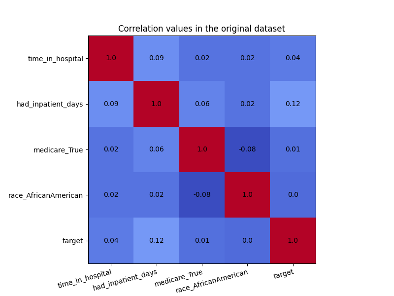
In the visualization below, we see the correlation values in the original dataset. We are particularly interested in the correlations between the ‘race_AfricanAmerican’ column and the three non-sensitive attributes ‘time_in_hospital’, ‘had_inpatient_days’ and ‘medicare_True’. The target variable is also included in these visualization for completeness, and it is defined as a binary feature which indicated whether the readmission of a patient occurred within 30 days of the release. We see that ‘race_AfricanAmerican’ is not highly correlated with the three mentioned attributes, but we want to remove these correlations nonetheless. The code for generating the correlation matrix can be found in this example notebook.

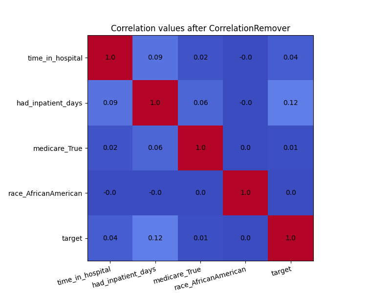
In order to see the effect of CorrelationRemover, we visualize how the correlation matrix has changed after the transformation of the dataset. Due to rounding, some of the 0.0 values appear as -0.0. Either way, the CorrelationRemover successfully removed all correlation between ‘race_AfricanAmerican’ and the other columns while retaining the correlation between the other features.

We can also use the alpha parameter with for instance \(\alpha=0.5\) to control the level of filtering between the sensitive and non-sensitive features.

>>> cr = CorrelationRemover(sensitive_feature_ids=['race_AfricanAmerican'], alpha=0.5)
>>> cr.fit(X)
CorrelationRemover(alpha=0.5, sensitive_feature_ids=['race_AfricanAmerican'])
>>> X_transform = cr.transform(X)

As we can see in the visulization below, not all correlation between ‘race_AfricanAmerican’ and the other columns was removed. This is exactly what we would expect with \(\alpha=0.5\).