2. Assessment

2.1. Metrics

The fairlearn.metrics module provides the means to assess fairness-related metrics for models. This applies for any kind of model that users may already use, but also for models created with mitigation techniques from the Mitigation section. The Fairlearn dashboard provides a visual way to compare metrics between models as well as compare metrics for different groups on a single model.

2.1.1. Ungrouped Metrics

At their simplest, metrics take a set of ‘true’ values \(Y_{true}\) (from the input data) and predicted values \(Y_{pred}\) (by applying the model to the input data), and use these to compute a measure. For example, the recall or true positive rate is given by

\[P( Y_{pred}=1 \given Y_{true}=1 )\]

That is, a measure of whether the model finds all the positive cases in the input data. The scikit-learn package implements this in sklearn.metrics.recall_score().

Suppose we have the following data we can see that the prediction is 1 in five of the ten cases where the true value is 1, so we expect the recall to be 0.5:

>>> import sklearn.metrics as skm
>>> Y_true = [0, 1, 1, 1, 1, 0, 1, 0, 1, 0, 0, 0, 1, 1, 1, 1]
>>> Y_pred = [0, 0, 1, 0, 1, 1, 1, 0, 0, 1, 1, 1, 1, 0, 0, 1]
>>> skm.recall_score(Y_true, Y_pred)
0.5

2.1.2. Metrics with Grouping

When considering fairness, each row of input data will have an associated group label \(g \in G\), and we will want to know how the metric behaves for each \(g\). To help with this, Fairlearn provides a class, which takes an existing (ungrouped) metric function, and applies it to each group within a set of data.

Suppose in addition to the \(Y_{true}\) and \(Y_{pred}\) above, we had the following set of labels:

>>> import numpy as np
>>> import pandas as pd
>>> group_membership_data = ['d', 'a', 'c', 'b', 'b', 'c', 'c', 'c',
...                          'b', 'd', 'c', 'a', 'b', 'd', 'c', 'c']
>>> pd.set_option('display.max_columns', 20)
>>> pd.set_option('display.width', 80)
>>> pd.DataFrame({ 'Y_true': Y_true,
...                'Y_pred': Y_pred,
...                'group_membership_data': group_membership_data})
    Y_true  Y_pred group_membership_data
0        0       0                     d
1        1       0                     a
2        1       1                     c
3        1       0                     b
4        1       1                     b
5        0       1                     c
6        1       1                     c
7        0       0                     c
8        1       0                     b
9        0       1                     d
10       0       1                     c
11       0       1                     a
12       1       1                     b
13       1       0                     d
14       1       0                     c
15       1       1                     c

We then calculate a metric which shows the subgroups:

>>> from fairlearn.metrics import MetricFrame
>>> grouped_metric = MetricFrame(skm.recall_score,
...                              Y_true, Y_pred,
...                              sensitive_features=group_membership_data)
>>> print("Overall recall = ", grouped_metric.overall)
Overall recall =  0.5
>>> print("recall by groups = ", grouped_metric.by_group.to_dict())
recall by groups =  {'a': 0.0, 'b': 0.5, 'c': 0.75, 'd': 0.0}

Note that the overall recall is the same as that calculated above in the Ungrouped Metric section, while the ‘by group’ dictionary can be checked against the table above.

In addition to these basic scores, Fairlearn also provides convenience functions to recover the maximum and minimum values of the metric across groups and also the difference and ratio between the maximum and minimum:

>>> print("min recall over groups = ", grouped_metric.group_min())
min recall over groups =  0.0
>>> print("max recall over groups = ", grouped_metric.group_max())
max recall over groups =  0.75
>>> print("difference in recall = ", grouped_metric.difference(method='between_groups'))
difference in recall =  0.75
>>> print("ratio in recall = ", grouped_metric.ratio(method='between_groups'))
ratio in recall =  0.0

A single instance of fairlearn.metrics.MetricFrame can evaluate multiple metrics simultaneously:

>>> multi_metric = MetricFrame({'precision':skm.precision_score, 'recall':skm.recall_score},
...                             Y_true, Y_pred,
...                             sensitive_features=group_membership_data)
>>> multi_metric.overall
precision    0.555556
recall            0.5
dtype: object
>>> multi_metric.by_group
     precision recall
sensitive_feature_0
a            0      0
b            1    0.5
c          0.6   0.75
d            0      0

If there are per-sample arguments (such as sample weights), these can also be provided in a dictionary via the sample_params argument.:

>>> s_w = [1, 2, 1, 3, 2, 3, 1, 2, 1, 2, 3, 1, 2, 3, 2, 3]
>>> s_p = { 'sample_weight':s_w }
>>> weighted = MetricFrame(skm.recall_score,
...                        Y_true, Y_pred,
...                        sensitive_features=pd.Series(group_membership_data, name='SF 0'),
...                        sample_params=s_p)
>>> weighted.overall
0.45
>>> weighted.by_group
SF 0
a               0
b             0.5
c        0.714286
d               0
Name: recall_score, dtype: object

If mutiple metrics are being evaluated, then sample_params becomes a dictionary of dictionaries, with the first key corresponding matching that in the dictionary holding the desired underlying metric functions.

We do not support non-sample parameters at the current time. If these are required, then use functools.partial() to prebind the required arguments to the metric function:

>>> import functools
>>> fbeta_06 = functools.partial(skm.fbeta_score, beta=0.6)
>>> metric_beta = MetricFrame(fbeta_06,
...                           Y_true, Y_pred,
...                           sensitive_features=group_membership_data)
>>> metric_beta.overall
0.5396825396825397
>>> metric_beta.by_group
sensitive_feature_0
a            0
b     0.790698
c      0.63354
d            0
Name: metric, dtype: object

Finally, multiple sensitive features can be specified. The by_groups property then holds the intersections of these groups:

>>> g_2 = [ 8,6,8,8,8,8,6,6,6,8,6,6,6,6,8,6]
>>> s_f_frame = pd.DataFrame(np.stack([group_membership_data, g_2], axis=1),
...                          columns=['SF 0', 'SF 1'])
>>> metric_2sf = MetricFrame(skm.recall_score,
...                          Y_true, Y_pred,
...                          sensitive_features=s_f_frame)
>>> metric_2sf.overall  # Same as before
0.5
>>> metric_2sf.by_group
SF 0  SF 1
a     6         0
      8       NaN
b     6       0.5
      8       0.5
c     6         1
      8       0.5
d     6         0
      8         0
Name: recall_score, dtype: object

With such a small number of samples, we are obviously running into cases where there are no members in a particular combination of sensitive features. In this case we see that the subgroup (a, 8) has a result of NaN, indicating that there were no samples in it.

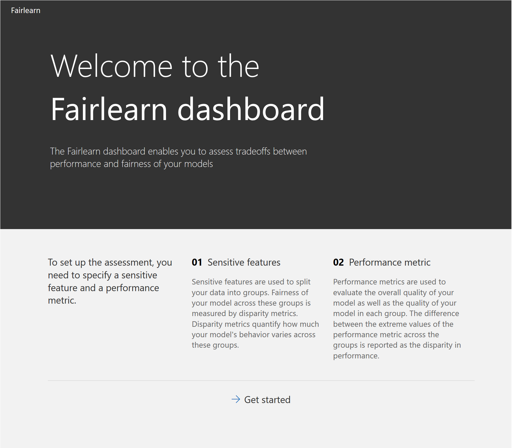
2.2. Fairlearn dashboard

The Fairlearn dashboard is a Jupyter notebook widget for assessing how a model’s predictions impact different groups (e.g., different ethnicities), and also for comparing multiple models along different fairness and performance metrics.

Note

The FairlearnDashboard will move from Fairlearn to the raiwidgets package after the v0.5.0 release. Instead, Fairlearn will provide some of the existing functionality through matplotlib-based visualizations.

2.2.1. Setup and a single-model assessment

To assess a single model’s fairness and performance, the dashboard widget can be launched within a Jupyter notebook as follows:

from fairlearn.widget import FairlearnDashboard

# A_test containts your sensitive features (e.g., age, binary gender)
# sensitive_feature_names contains your sensitive feature names
# y_true contains ground truth labels
# y_pred contains prediction labels

FairlearnDashboard(sensitive_features=A_test,
                   sensitive_feature_names=['BinaryGender', 'Age'],
                   y_true=Y_test.tolist(),
                   y_pred=[y_pred.tolist()])

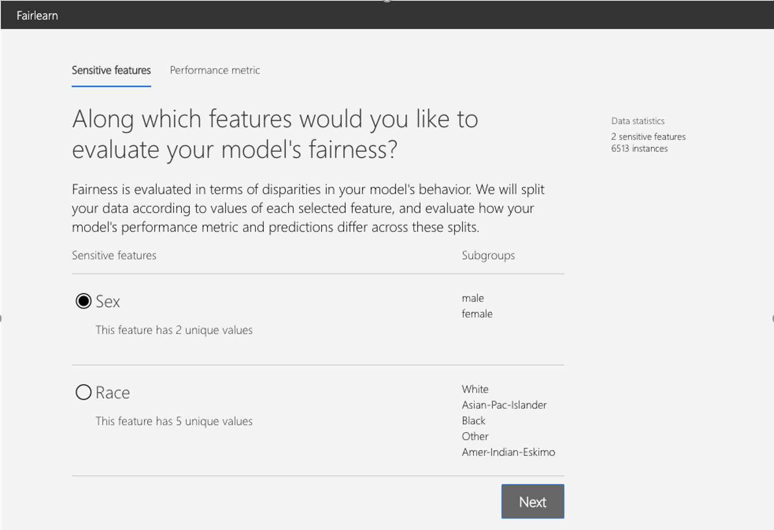
After the launch, the widget walks the user through the assessment setup, where the user is asked to select

1. the sensitive feature of interest (e.g., binary gender or age), and

2. the performance metric (e.g., model precision) along which to evaluate the overall model performance as well as any disparities across groups. These selections are then used to obtain the visualization of the model’s impact on the subgroups (e.g., model precision for females and model precision for males).

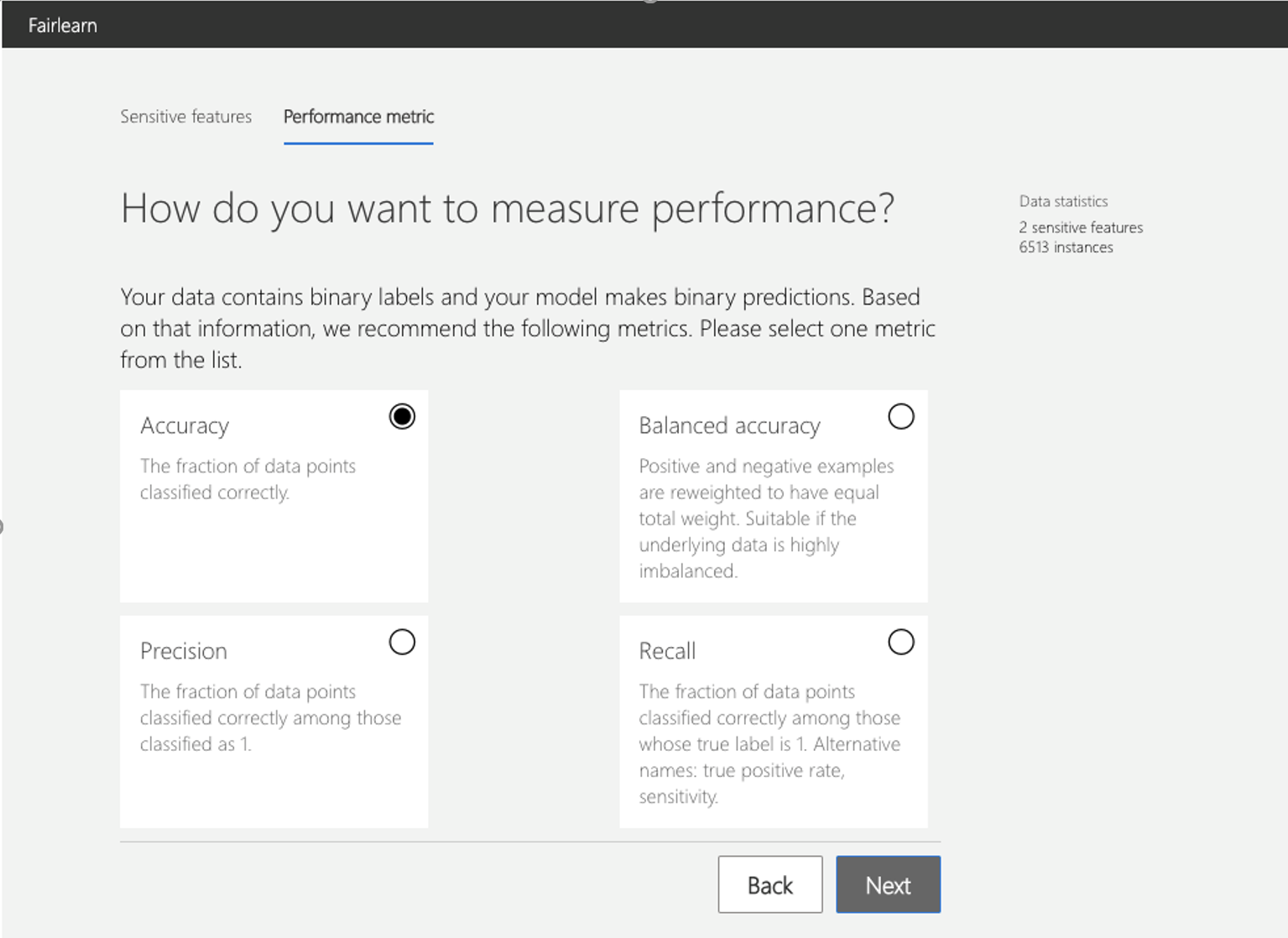
The following figures illustrate the setup steps, where binary gender is selected as a sensitive feature and accuracy rate is selected as the performance metric.

After the setup, the dashboard presents the model assessment in two panels:

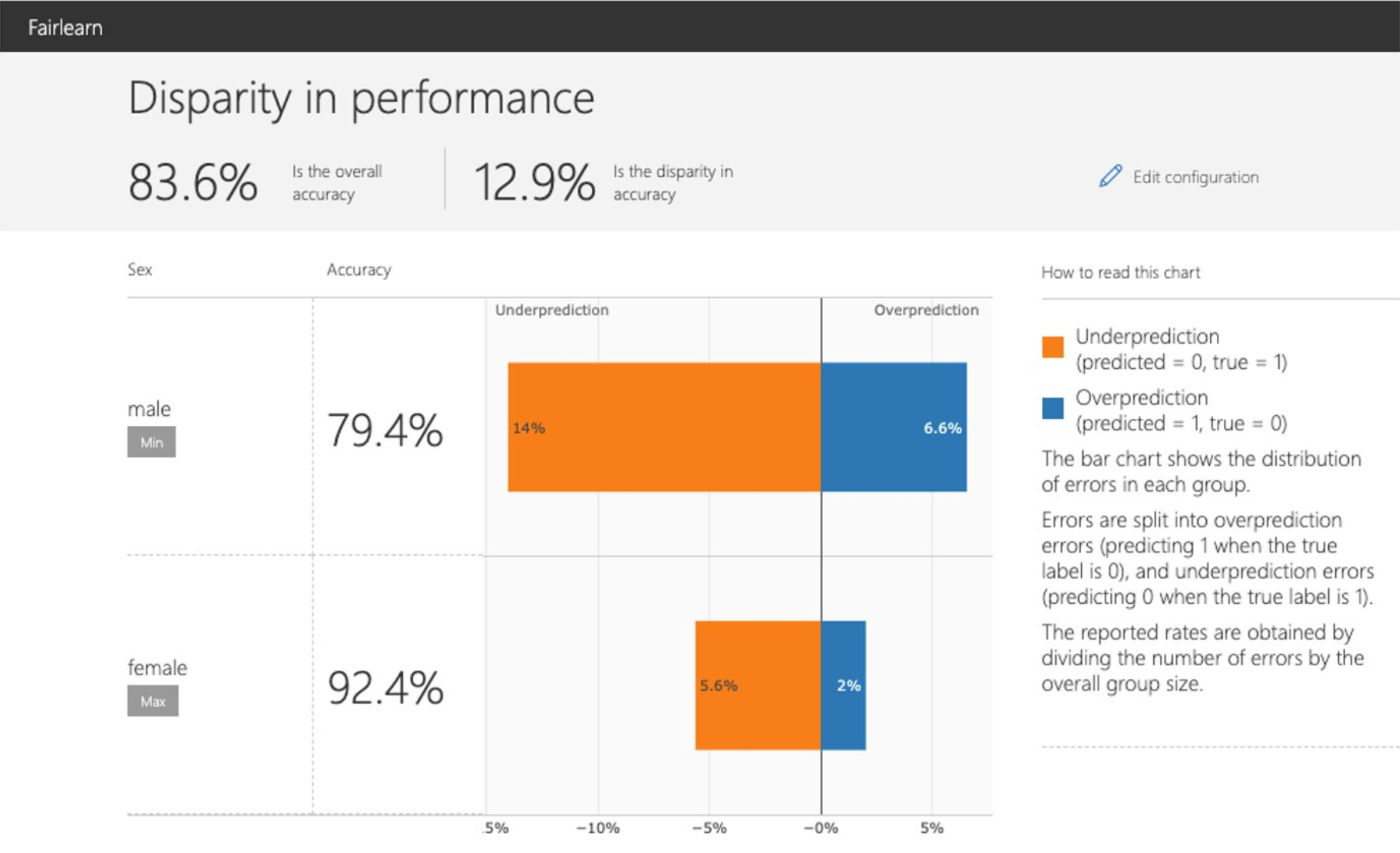
Disparity in performance

This panel shows: (1) the performance of your model with respect to your selected performance metric (e.g., accuracy rate) overall as well as on different subgroups based on your selected sensitive feature (e.g., accuracy rate for females, accuracy rate for males); (2) the disparity (difference) in the values of the selected performance metric across different subgroups; (3) the distribution of errors in each subgroup (e.g., female, male). For binary classification, the errors are further split into overprediction (predicting 1 when the true label is 0), and underprediction (predicting 0 when the true label is 1).

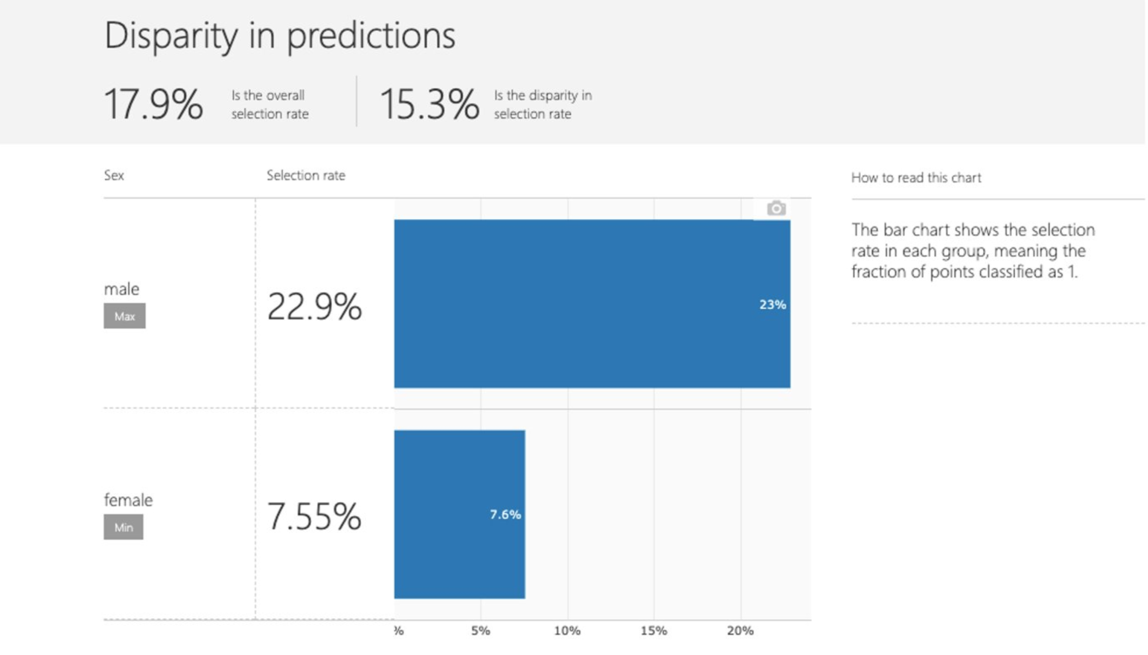
Disparity in predictions

This panel shows a bar chart that contains the selection rate in each group, meaning the fraction of data classified as 1 (in binary classification) or distribution of prediction values (in regression).

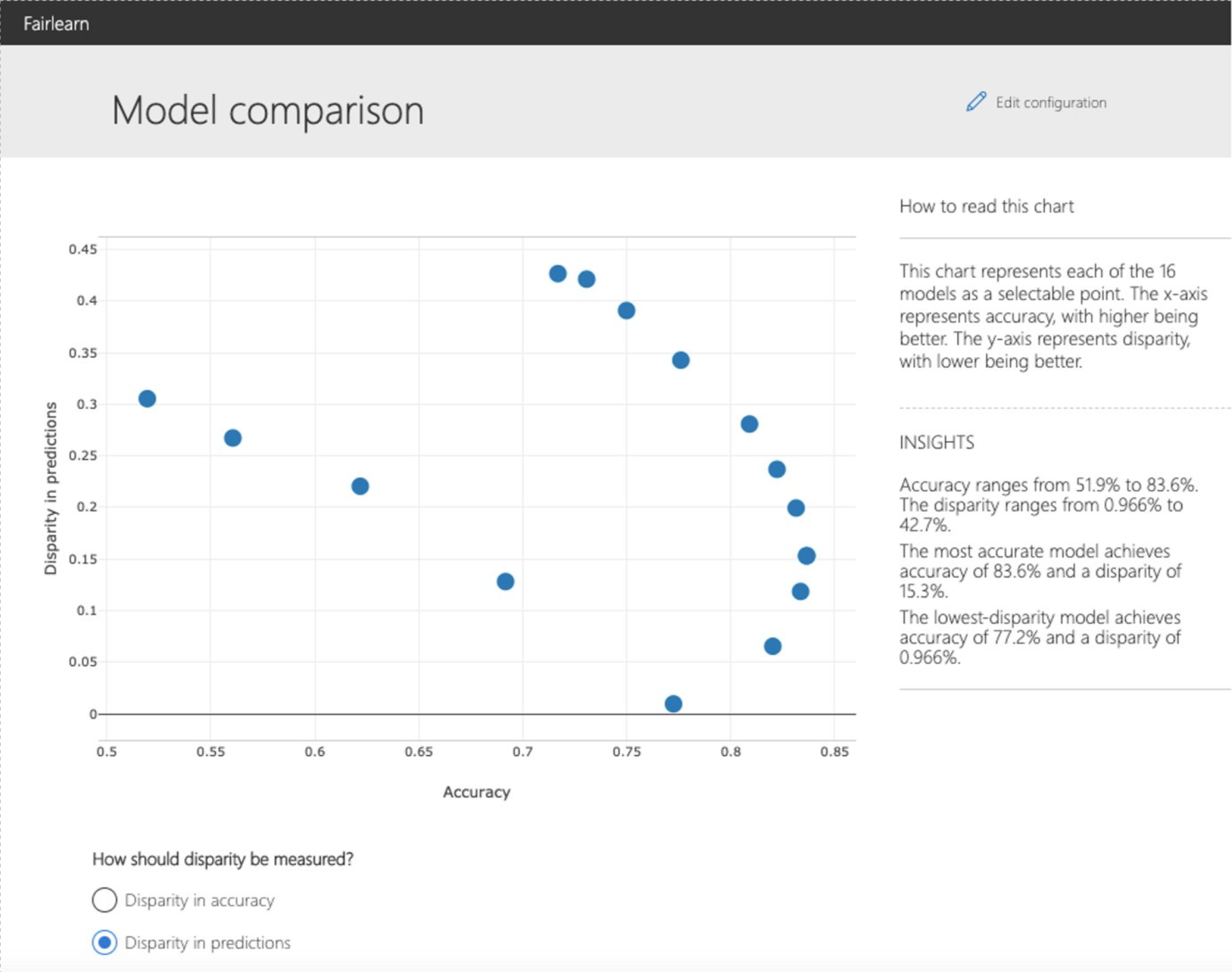
2.2.2. Comparing multiple models

The dashboard also enables comparison of multiple models, such as the models produced by different learning algorithms and different mitigation approaches, including fairlearn.reductions.GridSearch, fairlearn.reductions.ExponentiatedGradient, and fairlearn.postprocessing.ThresholdOptimizer.

As before, the user is first asked to select the sensitive feature and the performance metric. The model comparison view then depicts the performance and disparity of all the provided models in a scatter plot. This allows the user to examine trade-offs between performance and fairness. Each of the dots can be clicked to open the assessment of the corresponding model. The figure below shows the model comparison view with binary gender selected as a sensitive feature and accuracy rate selected as the performance metric.