Preprocessing

Preprocessing algorithms transform the dataset to mitigate possible unfairness present in the data. Preprocessing algorithms in Fairlearn follow the sklearn.base.TransformerMixin class, meaning that they can fit to the dataset and transform it (or fit_transform to fit and transform in one go).

Correlation Remover

Sensitive features can be correlated with non-sensitive features in the dataset. By applying the CorrelationRemover, these correlations are projected away while details from the original data are retained as much as possible (as measured by the least-squares error). The user can control the level of projection via the alpha parameter.

In mathematical terms, assume we have the original dataset \(\mathbf{X}\), which contains a set of sensitive features denoted by \(\mathbf{S}\) and a set of non-sensitive features denoted by \(\mathbf{Z}\). The goal is to remove correlations between the sensitive features and the non-sensitive features.

Let \(m_s\) and \(m_{ns}\) denote the number of sensitive and non-sensitive features, respectively. Let \(\bar{\mathbf{s}}\) represent the mean of the sensitive features, i.e., \(\bar{\mathbf{s}} = [\bar{s}_1, \dots, \bar{s}_{m_s}]^\top\), where \(\bar{s}_j\) is the mean of the \(j\text{-th}\) sensitive feature.

For each non-sensitive feature \(\mathbf{z}_j\in\mathbb{R}^n\), where \(j=1,\dotsc,m_{ns}\), we compute an optimal weight vector \(\mathbf{w}_j^* \in \mathbb{R}^{m_s}\) that minimizes the following least squares objective:

\[\min _{\mathbf{w}} \| \mathbf{z}_j - (\mathbf{S}-\mathbf{1}_n\times\bar{\mathbf{s}}^\top) \mathbf{w} \|_2^2\]

where \(\mathbf{1}_n\) is the all-one vector in \(\mathbb{R}^n\).

In other words, \(\mathbf{w}_j^*\) is the solution to a linear regression problem where we project \(\mathbf{z}_j\) onto the centered sensitive features. The weight matrix \(\mathbf{W}^* = (\mathbf{w}_1^*, \dots, \mathbf{w}_{m_{ns}}^*)\) is thus obtained by solving this regression for each non-sensitive feature.

Once we have the optimal weight matrix \(\mathbf{W}^*\), we compute the residual non-sensitive features \(\mathbf{Z}^*\) as follows:

\[\mathbf{Z}^* = \mathbf{Z} - (\mathbf{S}-\mathbf{1}_n\times\bar{\mathbf{s}}^\top) \mathbf{W}^*\]

The columns in \(\mathbf{S}\) will be dropped from the dataset \(\mathbf{X}\), and \(\mathbf{Z}^*\) will replace the original non-sensitive features \(\mathbf{Z}\), but the hyper parameter \(\alpha\) does allow you to tweak the amount of filtering that gets applied:

\[\mathbf{X}_{\text{tfm}} = \alpha \mathbf{X}_{\text{filtered}} + (1-\alpha) \mathbf{X}_{\text{orig}}\]

Note that the lack of correlation does not imply anything about statistical dependence. In particular, since correlation measures linear relationships, it might still be possible that non-linear relationships exist in the data. Therefore, we expect this to be most appropriate as a preprocessing step for (generalized) linear models.

In the example below, the Diabetes 130-Hospitals is loaded and the correlation between the African American race and the non-sensitive features is removed. This dataset contains more races, but in example we will only focus on the African American race. The CorrelationRemover will drop the sensitive features from the dataset.

>>> from fairlearn.preprocessing import CorrelationRemover
>>> import pandas as pd
>>> from fairlearn.datasets import fetch_diabetes_hospital
>>> data = fetch_diabetes_hospital()
>>> X = data.data[["race", "time_in_hospital", "had_inpatient_days", "medicare"]]
>>> X = pd.get_dummies(X)
>>> X = X.drop(["race_Asian",
...                     "race_Caucasian",
...                     "race_Hispanic",
...                     "race_Other",
...                     "race_Unknown",
...                     "had_inpatient_days_False",
...                     "medicare_False"], axis=1)
>>> cr = CorrelationRemover(sensitive_feature_ids=['race_AfricanAmerican'])
>>> cr.fit(X)
CorrelationRemover(sensitive_feature_ids=['race_AfricanAmerican'])
>>> X_transform = cr.transform(X)

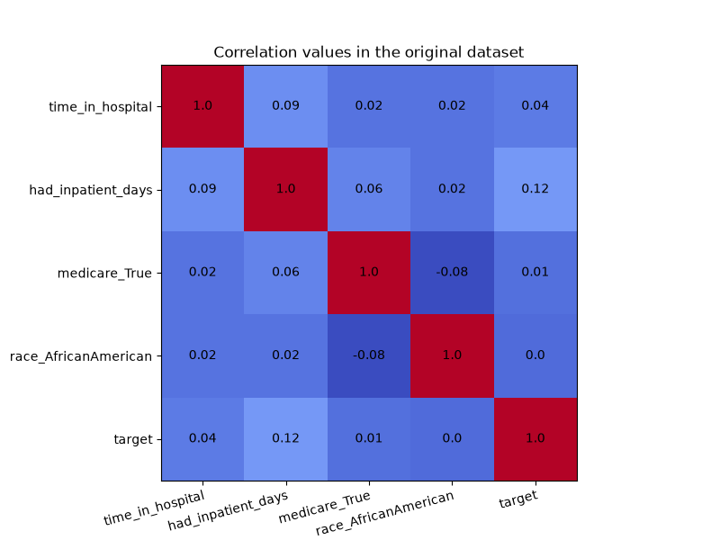
In the visualization below, we see the correlation values in the original dataset. We are particularly interested in the correlations between the ‘race_AfricanAmerican’ column and the three non-sensitive features ‘time_in_hospital’, ‘had_inpatient_days’ and ‘medicare_True’. The target variable is also included in these visualization for completeness, and it is defined as a binary feature which indicated whether the readmission of a patient occurred within 30 days of the release. We see that ‘race_AfricanAmerican’ is not highly correlated with the three mentioned features, but we want to remove these correlations nonetheless. The code for generating the correlation matrix can be found in this example notebook.

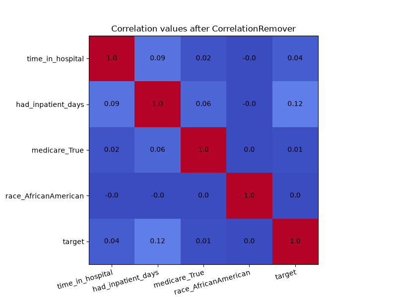
In order to see the effect of CorrelationRemover, we visualize how the correlation matrix has changed after the transformation of the dataset. Due to rounding, some of the 0.0 values appear as -0.0. Either way, the CorrelationRemover successfully removed all correlation between ‘race_AfricanAmerican’ and the other columns while retaining the correlation between the other features.

We can also use the alpha parameter with for instance \(\alpha=0.5\) to control the level of filtering between the sensitive and non-sensitive features.

>>> cr = CorrelationRemover(sensitive_feature_ids=['race_AfricanAmerican'], alpha=0.5)
>>> cr.fit(X)
CorrelationRemover(alpha=0.5, sensitive_feature_ids=['race_AfricanAmerican'])
>>> X_transform = cr.transform(X)

As we can see in the visualization below, not all correlation between ‘race_AfricanAmerican’ and the other columns was removed. This is exactly what we would expect with \(\alpha=0.5\).

Prototype Representation Learner

PrototypeRepresentationLearner is a preprocessing algorithm and a classifier that aims to learn a latent representation of the data that minimizes reconstruction error, while simultaneously obfuscating information about sensitive features. It was introduced in Zemel et al. (2013) [1].

The latent representation consists of \(K\) prototype vectors \(\mathbf{v}_1, \dots, \mathbf{v}_K \in \mathbb{R}^d\), where \(d\) is the dimension of the input data, and a stochastic transformation matrix \(\mathbf{M} \in \mathbb{R}^{n \times k}\) that maps the input data \(\mathbf{X} \in \mathbb{R}^{n \times d}\) to the prototypes. Each entry \(M_{nk}\) is the softmax of the distances of the sample \(n\) to the prototype vectors:

\[M_{nk} = \frac{\exp(-d(\mathbf{x}_n, \mathbf{v}_k))}{\sum_{k'=1}^{K} \exp(-d(\mathbf{x}_n, \mathbf{v}_{k'}))}\]

The algorithm works by solving an optimization problem that balances the trade-off between classification accuracy, group and individual fairness, and reconstruction error. The objective function is thus defined as a weighted sum of three terms:

\[\text{reconstruct_weight} \times L_x + \text{target_weight} \times L_y + \text{fairness_weight} \times L_z\]

where:

\(L_x\) is the reconstruction error term that writes as:

\[L_x = \frac{1}{N} \sum_{n=1}^{N} \| \mathbf{x}_n - \hat{\mathbf{x}}_n \|_2^2\]

\(L_y\) is the classification error term that is equal to the log loss:

\[L_y = -\frac{1}{N} \sum_{n=1}^{N} y_n \log(\hat{y}_n) + (1-y_n) \log(1-\hat{y}_n)\]

\(L_z\) is the demographic parity difference’s approximation term that is defined as:

\[L_z = \frac{1}{K \times \binom{G}{2}} \sum_{k=1}^{K} \sum_{g < g'} \left| M_{gk} - M_{g'k} \right|\]

where \(1\leq g, g'\leq G\) are the indices of the groups in the sensitive features and \(M_{gk}\) is the average of the entries of the transformation matrix \(\mathbf{M}\) for group \(g\) and prototype \(k\).

In the example below, we use the Adult Income dataset to demonstrate the PrototypeRepresentationLearner. This dataset contains sensitive features such as race and sex. The goal is to transform the dataset so that the sensitive features have less influence on the predictions of a downstream model.

>>> from fairlearn.preprocessing import PrototypeRepresentationLearner
>>> from fairlearn.datasets import fetch_adult
>>> from sklearn.model_selection import train_test_split
>>> from sklearn.preprocessing import StandardScaler
>>> import pandas as pd
>>> features_to_keep = ["fnlwgt", "capital-gain", "capital-loss", "hours-per-week", "age"]
>>> senstive_feature_id = "race_White"
>>> raw_data = fetch_adult().frame
>>> data, target = (
...     raw_data[features_to_keep + ["race"]],
...     raw_data["class"] == ">50K",
... )
>>> data = pd.get_dummies(data)
>>> data, sensitive_features = data[features_to_keep], data[senstive_feature_id]
>>> X_train, X_test, y_train, y_test, sf_train, sf_test = train_test_split(
...     data, target, sensitive_features, test_size=0.3, random_state=42
... )
>>> scaler = StandardScaler()
>>> X_train = scaler.fit_transform(X_train)
>>> X_test = scaler.transform(X_test)
>>> prl = PrototypeRepresentationLearner(n_prototypes=4, max_iter=10)
>>> prl.fit(X_train, y_train, sensitive_features=sf_train)
PrototypeRepresentationLearner(max_iter=10, n_prototypes=4)
>>> X_train_transformed = prl.transform(X_train)
>>> X_test_transformed = prl.transform(X_test)
>>> y_hat = prl.predict(X_test)

Note that when used solely as a transformer, the PrototypeRepresentationLearner does not require the target labels to be passed to the fit method; they are only required when the PrototypeRepresentationLearner is used as a classifier. In case they are not provided, the classification error term will not be included in the loss function, and the predict method will raise an exception when called.

>>> prl = PrototypeRepresentationLearner(n_prototypes=4, max_iter=10)
>>> prl.fit(X_train, sensitive_features=sf_train)
PrototypeRepresentationLearner(max_iter=10, n_prototypes=4)
>>> X_train_transformed = prl.transform(X_train)
>>> X_test_transformed = prl.transform(X_test)

References

[1]

Rich Zemel, Yu Wu, Kevin Swersky, Toni Pitassi, and Cynthia Dwork. Learning fair representations. In Sanjoy Dasgupta and David McAllester, editors, Proceedings of the 30th International Conference on Machine Learning, volume 28 of Proceedings of Machine Learning Research, 325–333. Atlanta, Georgia, USA, 17–19 Jun 2013. PMLR. URL: https://proceedings.mlr.press/v28/zemel13.html.