

Note
Go to the end to download the full example code. or to run this example in your browser via JupyterLite
GridSearch with Census Data#
Census dataset. This dataset is a classification problem - given a range of data about 32,000 individuals, predict whether their annual income is above or below fifty thousand dollars per year.
For the purposes of this notebook, we shall treat this as a loan decision problem. We will pretend that the label indicates whether or not each individual repaid a loan in the past. We will use the data to train a predictor to predict whether previously unseen individuals will repay a loan or not. The assumption is that the model predictions are used to decide whether an individual should be offered a loan.
We will first train a fairness-unaware predictor and show that it leads to unfair
decisions under a specific notion of fairness called demographic parity.
We then mitigate unfairness by applying the GridSearch algorithm from the
Fairlearn package.
Load and preprocess the data set#
We download the data set using fetch_adult function in fairlearn.datasets. We start by importing the various modules we’re going to use:
import matplotlib.pyplot as plt
import pandas as pd
from sklearn import metrics as skm
from sklearn.linear_model import LogisticRegression
from sklearn.model_selection import train_test_split
from sklearn.preprocessing import LabelEncoder, StandardScaler

from fairlearn.datasets import fetch_adult
from fairlearn.metrics import (
    MetricFrame,
    count,
    plot_model_comparison,
    selection_rate,
    selection_rate_difference,
)
from fairlearn.reductions import DemographicParity, ErrorRate, GridSearch
We can now load and inspect the data by using the fairlearn.datasets module:
data = fetch_adult()
X_raw = data.data
Y = (data.target == ">50K") * 1
X_raw
We are going to treat the sex of each individual as a sensitive feature (where 0 indicates female and 1 indicates male), and in this particular case we are going separate this feature out and drop it from the main data. We then perform some standard data preprocessing steps to convert the data into a format suitable for the ML algorithms
A = X_raw["sex"]
X = X_raw.drop(labels=["sex"], axis=1)
X = pd.get_dummies(X)

sc = StandardScaler()
X_scaled = sc.fit_transform(X)
X_scaled = pd.DataFrame(X_scaled, columns=X.columns)

le = LabelEncoder()
Y = le.fit_transform(Y)
Finally, we split the data into training and test sets:
X_train, X_test, Y_train, Y_test, A_train, A_test = train_test_split(
    X_scaled, Y, A, test_size=0.4, random_state=0, stratify=Y
)

# Work around indexing bug
X_train = X_train.reset_index(drop=True)
A_train = A_train.reset_index(drop=True)
X_test = X_test.reset_index(drop=True)
A_test = A_test.reset_index(drop=True)
Training a fairness-unaware predictor#
To show the effect of Fairlearn we will first train a standard ML predictor
that does not incorporate fairness. For speed of demonstration, we use the
simple sklearn.linear_model.LogisticRegression class:
unmitigated_predictor = LogisticRegression(solver="liblinear", fit_intercept=True)

unmitigated_predictor.fit(X_train, Y_train)
We can start to assess the predictor’s fairness using the MetricFrame:
metric_frame = MetricFrame(
    metrics={
        "accuracy": skm.accuracy_score,
        "selection_rate": selection_rate,
        "count": count,
    },
    sensitive_features=A_test,
    y_true=Y_test,
    y_pred=unmitigated_predictor.predict(X_test),
)
print(metric_frame.overall)
print(metric_frame.by_group)
metric_frame.by_group.plot.bar(
    subplots=True,
    layout=[3, 1],
    legend=False,
    figsize=[12, 8],
    title="Accuracy and selection rate by group",
)
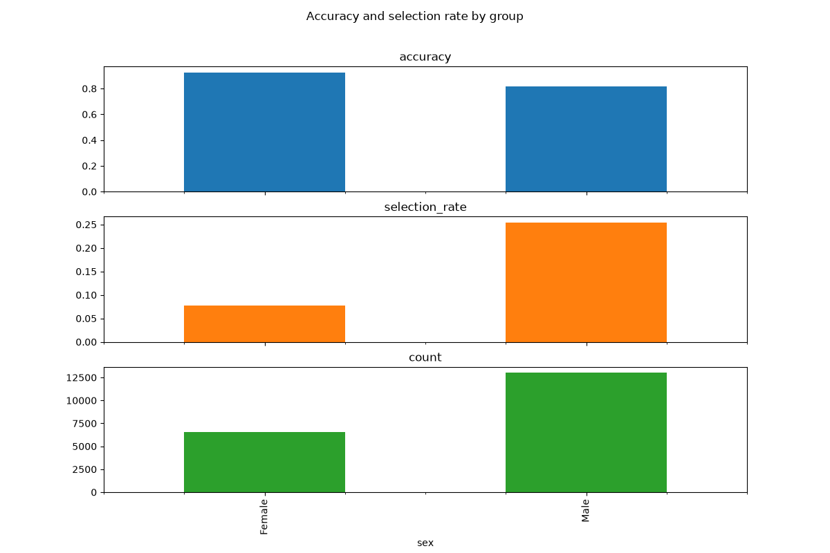
accuracy              0.851820
selection_rate        0.194707
count             19537.000000
dtype: float64
        accuracy  selection_rate    count
sex
Female  0.925960        0.076794   6537.0
Male    0.814538        0.254000  13000.0

array([[<Axes: title={'center': 'accuracy'}, xlabel='sex'>],
       [<Axes: title={'center': 'selection_rate'}, xlabel='sex'>],
       [<Axes: title={'center': 'count'}, xlabel='sex'>]], dtype=object)
Looking at the disparity in accuracy, we see that males have an error about three times greater than the females. More interesting is the disparity in opportunity - males are offered loans at three times the rate of females.
Despite the fact that we removed the feature from the training data, our predictor still discriminates based on sex. This demonstrates that simply ignoring a sensitive feature when fitting a predictor rarely eliminates unfairness. There will generally be enough other features correlated with the removed feature to lead to disparate impact.
Mitigation with GridSearch#
The fairlearn.reductions.GridSearch class implements a simplified
version of the exponentiated gradient reduction of Agarwal et al.
[1]. The user supplies a standard ML
estimator, which is treated as a blackbox. GridSearch works by generating a
sequence of relabellings and reweightings, and trains a predictor for each.
For this example, we specify demographic parity (on the sensitive feature of sex) as the fairness metric. Demographic parity requires that individuals are offered the opportunity (are approved for a loan in this example) independent of membership in the sensitive class (i.e., females and males should be offered loans at the same rate). We are using this metric for the sake of simplicity; in general, the appropriate fairness metric will not be obvious.
sweep = GridSearch(
    LogisticRegression(solver="liblinear", fit_intercept=True),
    constraints=DemographicParity(),
    grid_size=31,
)
Our algorithms provide fit() and predict() methods, so they
behave in a similar manner to other ML packages in Python. We do however have
to specify two extra arguments to fit() - the column of sensitive
feature labels, and also the number of predictors to generate in our sweep.
After fit() completes, we extract the full set of predictors from the
fairlearn.reductions.GridSearch object.
sweep.fit(X_train, Y_train, sensitive_features=A_train)

predictors = sweep.predictors_
We could plot performance and fairness metrics of these predictors now. However, the plot would be somewhat confusing due to the number of models. In this case, we are going to remove the predictors which are dominated in the error-disparity space by others from the sweep (note that the disparity will only be calculated for the sensitive feature; other potentially sensitive features will not be mitigated). In general, one might not want to do this, since there may be other considerations beyond the strict optimization of error and disparity (of the given sensitive feature).
errors, disparities = [], []
for m in predictors:

    def classifier(X):
        return m.predict(X)

    error = ErrorRate()
    error.load_data(X_train, pd.Series(Y_train), sensitive_features=A_train)
    disparity = DemographicParity()
    disparity.load_data(X_train, pd.Series(Y_train), sensitive_features=A_train)

    errors.append(error.gamma(classifier).iloc[0])
    disparities.append(disparity.gamma(classifier).max())

all_results = pd.DataFrame({"predictor": predictors, "error": errors, "disparity": disparities})

non_dominated = []
for row in all_results.itertuples():
    errors_for_lower_or_eq_disparity = all_results["error"][
        all_results["disparity"] <= row.disparity
    ]
    if row.error <= errors_for_lower_or_eq_disparity.min():
        non_dominated.append(row.predictor)
Finally, we can evaluate the dominant models along with the unmitigated model.
predictions = {"unmitigated": unmitigated_predictor.predict(X_test)}
metric_frames = {"unmitigated": metric_frame}
for i in range(len(non_dominated)):
key = "dominant_model_{0}".format(i)
predictions[key] = non_dominated[i].predict(X_test)
metric_frames[key] = MetricFrame(
metrics={
"accuracy": skm.accuracy_score,
"selection_rate": selection_rate,
"count": count,
},
sensitive_features=A_test,
y_true=Y_test,
y_pred=predictions[key],
)
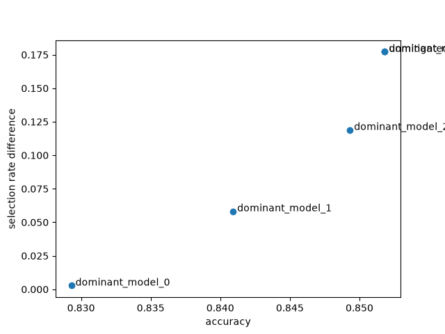
x = [metric_frame.overall["accuracy"] for metric_frame in metric_frames.values()]
y = [metric_frame.difference()["selection_rate"] for metric_frame in metric_frames.values()]
keys = list(metric_frames.keys())
plt.scatter(x, y)
for i in range(len(x)):
plt.annotate(keys[i], (x[i] + 0.0003, y[i]))
plt.xlabel("accuracy")
plt.ylabel("selection rate difference")
Text(24.722222222222214, 0.5, 'selection rate difference')
We see a Pareto front forming - the set of predictors which represent optimal tradeoffs between accuracy and disparity in predictions. In the ideal case, we would have a predictor at (1,0) - perfectly accurate and without any unfairness under demographic parity (with respect to the sensitive feature “sex”). The Pareto front represents the closest we can come to this ideal based on our data and choice of estimator. Note the range of the axes - the disparity axis covers more values than the accuracy, so we can reduce disparity substantially for a small loss in accuracy.
In a real example, we would pick the model which represented the best trade-off between accuracy and disparity given the relevant business constraints.
Comparing models easily#
Fairlearn also provides functionality to compare models much more easily.
# Plot model comparison
plot_model_comparison(
    x_axis_metric=skm.accuracy_score,
    y_axis_metric=selection_rate_difference,
    y_true=Y_test,
    y_preds=predictions,
    sensitive_features=A_test,
    point_labels=True,
    show_plot=True,
)
# End model comparison
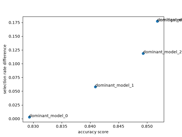
No matplotlib.Axes object was provided to draw on, so we create a new one

<Axes: xlabel='accuracy score', ylabel='selection rate difference'>
References#
Total running time of the script: (1 minutes 20.872 seconds)
Estimated memory usage: 263 MB