Plotting Metrics with Errors

import numpy as np
from sklearn.compose import ColumnTransformer
from sklearn.compose import make_column_selector as selector
from fairlearn.datasets import fetch_adult
from sklearn.impute import SimpleImputer
from sklearn.metrics import accuracy_score, confusion_matrix, recall_score
from sklearn.model_selection import train_test_split
from sklearn.pipeline import Pipeline
from sklearn.preprocessing import OneHotEncoder, StandardScaler
from sklearn.tree import DecisionTreeClassifier
from sklearn.utils import check_consistent_length

Load and preprocess the data set

We start by importing the various modules we’re going to use:

from fairlearn.experimental.enable_metric_frame_plotting import plot_metric_frame
from fairlearn.metrics import MetricFrame

We download the data set using the function fetch_adult() in fairlearn.datasets. The original Adult data set can be found at https://archive.ics.uci.edu/ml/datasets/Adult There are some caveats to using this dataset, but we will use it solely as an example to demonstrate the functionality of plotting metrics with error bars. We use a pipeline to preprocess the data then use a sklearn.tree.DecisionTreeClassifier to make predictions

data = fetch_adult()
X = data.data
y = (data.target == ">50K").astype(int)
X_train, X_test, y_train_true, y_test_true = train_test_split(
    X, y, test_size=0.33, random_state=42
)

numeric_transformer = Pipeline(
    steps=[
        ("impute", SimpleImputer()),
        ("scaler", StandardScaler()),
    ]
)

categorical_transformer = Pipeline(
    [
        ("impute", SimpleImputer(strategy="most_frequent")),
        ("ohe", OneHotEncoder(handle_unknown="ignore", sparse_output=False)),
    ]
)

preprocessor = ColumnTransformer(
    transformers=[
        ("num", numeric_transformer, selector(dtype_exclude="category")),
        ("cat", categorical_transformer, selector(dtype_include="category")),
    ]
)

complete_pipeline = Pipeline(
    [
        ("preprocessor", preprocessor),
        (
            "estimator",
            DecisionTreeClassifier(min_samples_leaf=10, max_depth=4),
        ),
    ]
)

complete_pipeline.fit(X_train, y_train_true)
y_test_pred = complete_pipeline.predict(X_test)
test_set_sex = X_test["race"]

Confidence interval calculations

We have many different choices for calculating confidence intervals. In this notebook we’ll just be using a Wilson score interval.

# We aim to create a 95% confidence interval, so we use a :code:`z_score` of 1.959964
z_score = 1.959964
digits_of_precision = 4
error_labels_legend = "95% Confidence Interval"


def general_wilson(p, n, digits=4, z=1.959964):
    """Return lower and upper bound of a Wilson confidence interval.

    Parameters
    ----------
    p : float
        Proportion of successes.
    n : int
        Total number of trials.
    digits : int
        Digits of precision to which the returned bound will be rounded
    z : float
        Z-score, which indicates the number of standard deviations of confidence.
        The default value of 1.959964 is for a 95% confidence interval

    Returns
    -------
        np.ndarray
        Array of length 2 of form: [lower_bound, upper_bound]
    """
    denominator = 1 + z**2 / n
    centre_adjusted_probability = p + z * z / (2 * n)
    adjusted_standard_deviation = np.sqrt((p * (1 - p) + z * z / (4 * n))) / np.sqrt(n)
    lower_bound = (
        centre_adjusted_probability - z * adjusted_standard_deviation
    ) / denominator
    upper_bound = (
        centre_adjusted_probability + z * adjusted_standard_deviation
    ) / denominator
    return np.array([round(lower_bound, digits), round(upper_bound, digits)])


def recall_wilson(y_true, y_pred):
    """Return a Wilson confidence interval for the recall metric.

    Parameters
    ----------
    y_true : array-like of shape (n_samples,)
        Ground truth labels
    y_pred : array-like of shape (n_samples,)
        Predicted labels

    Returns
    -------
        np.ndarray
        Array of length 2 of form: [lower_bound, upper_bound]
    """
    check_consistent_length(y_true, y_pred)
    tn, fp, fn, tp = confusion_matrix(y_true, y_pred).ravel()
    bounds = general_wilson(tp / (tp + fn), tp + fn, digits_of_precision, z_score)
    return bounds


def accuracy_wilson(y_true, y_pred):
    """Return a Wilson confidence interval for the accuracy metric.

    Parameters
    ----------
    y_true : array-like of shape (n_samples,)
        Ground truth labels
    y_pred : array-like of shape (n_samples,)
        Predicted labels

    Returns
    -------
        np.ndarray
        Array of length 2 of form: [lower_bound, upper_bound]
    """
    check_consistent_length(y_true, y_pred)
    score = accuracy_score(y_true, y_pred)
    bounds = general_wilson(score, len(y_true), digits_of_precision, z_score)
    return bounds

MetricFrame

Now we create a fairlearn.metrics.MetricFrame to generate the Wilson bounds for accuracy and recall

# Analyze metrics using :class:`fairlearn.metrics.MetricFrame`
metrics_dict = {
    "Recall": recall_score,
    "Recall Bounds": recall_wilson,
    "Accuracy": accuracy_score,
    "Accuracy Bounds": accuracy_wilson,
}
metric_frame = MetricFrame(
    metrics=metrics_dict,
    y_true=y_test_true,
    y_pred=y_test_pred,
    sensitive_features=test_set_sex,
)

Plotting

Plot metrics without confidence intervals

plot_metric_frame(metric_frame, kind="point", metrics=["Recall", "Accuracy"])

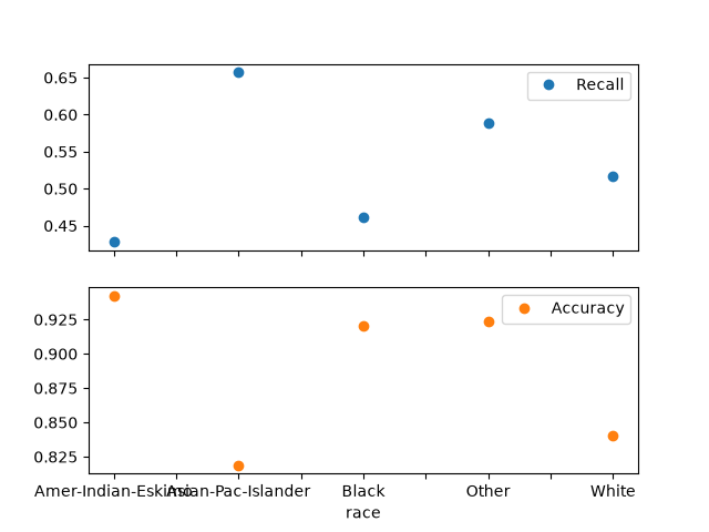
array([<Axes: xlabel='race'>, <Axes: xlabel='race'>], dtype=object)

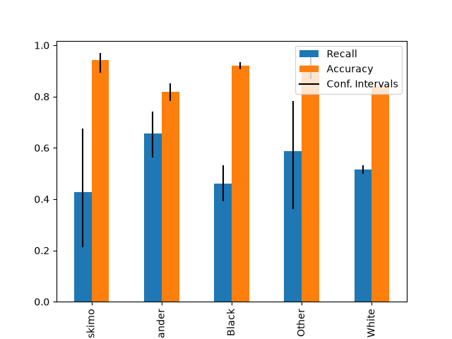
Plot metrics with confidence intervals (possibly asymmetric)

plot_metric_frame(
    metric_frame,
    kind="bar",
    metrics=["Recall", "Accuracy"],
    conf_intervals=["Recall Bounds", "Accuracy Bounds"],
    plot_ci_labels=True,
    subplots=False,
)
plot_metric_frame(
    metric_frame,
    kind="point",
    metrics="Recall",
    conf_intervals="Recall Bounds",
)

• 
• 

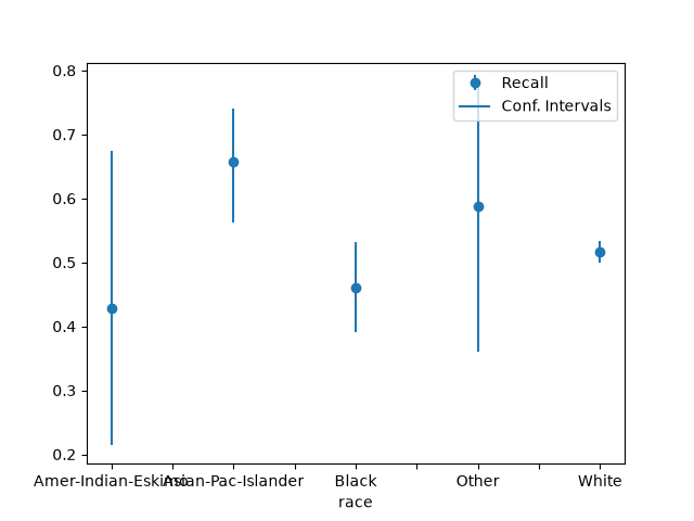
array([<Axes: xlabel='race'>], dtype=object)

Plot metrics with error labels

plot_metric_frame(
    metric_frame,
    kind="bar",
    metrics="Recall",
    conf_intervals="Recall Bounds",
    colormap="Pastel1",
    plot_ci_labels=True,
)

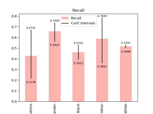
array([<Axes: title={'center': 'Recall'}, xlabel='race'>], dtype=object)

Plots all columns and treats them as metrics without error bars

plot_metric_frame(metric_frame, kind="bar", colormap="rainbow", layout=[1, 2])

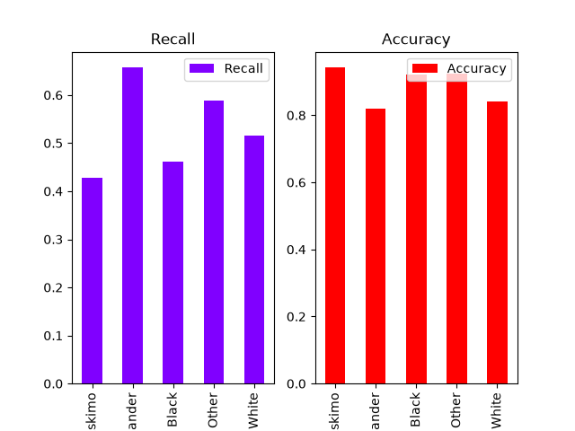
array([[<Axes: title={'center': 'Recall'}, xlabel='race'>,
        <Axes: title={'center': 'Accuracy'}, xlabel='race'>]],
      dtype=object)

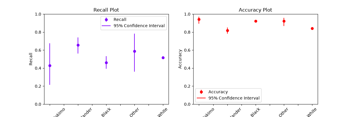
Customizing plots

plot_metric_frame() returns an Axes object that we can customize further.

axs = plot_metric_frame(
    metric_frame,
    kind="point",
    metrics=["Recall", "Accuracy"],
    conf_intervals=["Recall Bounds", "Accuracy Bounds"],
    subplots=True,
    ci_labels_legend=error_labels_legend,
    # the following parameters are passed into `pandas.DataFrame.plot` as kwargs
    layout=[1, 2],
    rot=45,
    colormap="rainbow",
    figsize=(12, 4),
)
axs[0][0].set_ylabel("Recall")
axs[0][0].set_title("Recall Plot")
axs[0][1].set_title("Accuracy Plot")
axs[0][0].set_xlabel("Race")
axs[0][1].set_xlabel("Race")
axs[0][0].set_ylabel("Recall")
axs[0][1].set_ylabel("Accuracy")

# Set the y-scale for both metrics to [0, 1]
axs[0][0].set_ylim((0, 1))
axs[0][1].set_ylim((0, 1))

(0.0, 1.0)